Simple and multiple regression#
Show code cell content
import numpy as np
import pandas as pd
# Safe setting for Pandas.  Needs Pandas version >= 1.5.
pd.set_option('mode.copy_on_write', True)

import matplotlib.pyplot as plt
plt.style.use('fivethirtyeight')

np.set_printoptions(suppress=True)
Show code cell content
def standard_units(any_numbers):
    """ Convert any array of numbers to standard units.
    """
    return (any_numbers - np.mean(any_numbers))/np.std(any_numbers)

def correlation(t, x, y):
    """ Correlation of columns `x` and `y` from data frame `t`
    """
    return np.mean(standard_units(t[x]) * standard_units(t[y]))
Back to simple regression#
The multiple regression page introduced an extension the simple regression methods we saw in the finding lines page, and those following.
Simple regression uses a single set of predictor values, and a straight line, to predict another set of values.
For example, in the finding lines page above, we predicted the “quality” scores (on the y-axis) from the “easiness” scores (on the x-axis).
Multiple regression takes this a step further. Now we use more than on sets of values to predict another set of values. For example, in the multiple regression page, we used many sets of values, such as first and second floor area, lot area, and others, in order to predict the house sale price.
The multiple regression page followed on directly from the classification pages; we used multiple regression to build a model of house prices, from the training set, and then predicted house prices in the testing set.
In this page we go back a little, to simple regression, and show how it relates to the multiple regression we have just done.
On the way, we will start using a standard statistics library in Python, called StatsModels.
Simple regression#
Let us return to simple regression - using one set of values (on the x axis) to predict another set of values (on the y axis).
Here is our familiar chronic kidney disease dataset.
ckd = pd.read_csv('ckd.csv')
ckd.head()
| Age | Blood Pressure | Specific Gravity | Albumin | Sugar | Red Blood Cells | Pus Cell | Pus Cell clumps | Bacteria | Blood Glucose Random | ... | Packed Cell Volume | White Blood Cell Count | Red Blood Cell Count | Hypertension | Diabetes Mellitus | Coronary Artery Disease | Appetite | Pedal Edema | Anemia | Class | |
|---|---|---|---|---|---|---|---|---|---|---|---|---|---|---|---|---|---|---|---|---|---|
| 0 | 48 | 70 | 1.005 | 4 | 0 | normal | abnormal | present | notpresent | 117 | ... | 32 | 6700 | 3.9 | yes | no | no | poor | yes | yes | 1 |
| 1 | 53 | 90 | 1.020 | 2 | 0 | abnormal | abnormal | present | notpresent | 70 | ... | 29 | 12100 | 3.7 | yes | yes | no | poor | no | yes | 1 |
| 2 | 63 | 70 | 1.010 | 3 | 0 | abnormal | abnormal | present | notpresent | 380 | ... | 32 | 4500 | 3.8 | yes | yes | no | poor | yes | no | 1 |
| 3 | 68 | 80 | 1.010 | 3 | 2 | normal | abnormal | present | present | 157 | ... | 16 | 11000 | 2.6 | yes | yes | yes | poor | yes | no | 1 |
| 4 | 61 | 80 | 1.015 | 2 | 0 | abnormal | abnormal | notpresent | notpresent | 173 | ... | 24 | 9200 | 3.2 | yes | yes | yes | poor | yes | yes | 1 |
5 rows × 25 columns
In our case, we restrict ourselves to the chronic kidney disease patients.
These patients have a 1 in the Class column.
We’re also going to restrict ourselves to looking at the following measures:
Serum Creatinine: a measure of how well the kidney is clearing substances from the blood. When creatinine is high, it means the kidney is not clearing well. This is the general measure of kidney disease that we are interested to predict.Blood Urea: another measure of the ability of the kidney to clear substances from the blood. Urea is high in the blood when the kidneys are not clearing efficiently.Hemoglobin: healthy kidneys release a hormone erythropoietin that stimulates production of red blood cells, and red blood cells contain the hemoglobin molecule. When the kidneys are damaged, they produce less erythropoietin, so the body produces fewer red blood cells, and there is a lower concentration of hemoglobin in the blood.
# Data frame restricted to kidney patients and columns of interest.
ckdp = ckd.loc[
    ckd['Class'] == 1,
    ['Serum Creatinine', 'Blood Urea', 'Hemoglobin']]
# Rename the columns with shorted names.
ckdp.columns = ['Creatinine', 'Urea', 'Hemoglobin']
ckdp.head()
| Creatinine | Urea | Hemoglobin | |
|---|---|---|---|
| 0 | 3.8 | 56 | 11.2 |
| 1 | 7.2 | 107 | 9.5 |
| 2 | 2.7 | 60 | 10.8 |
| 3 | 4.1 | 90 | 5.6 |
| 4 | 3.9 | 148 | 7.7 |
Why did we rename the columns? Because Statsmodels, by default, has problems with columns with spaces. See that page for why, and ways you can fix the problems.
First let us look at the relationship of the urea levels and the creatinine:
ckdp.plot.scatter('Urea', 'Creatinine')
<Axes: xlabel='Urea', ylabel='Creatinine'>
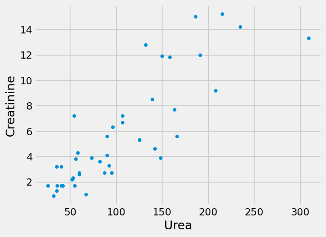
There is a positive correlation between these sets of values; high urea and high creatinine go together; both reflect the failure of the kidneys to clear substances from the blood.
correlation(ckdp, 'Urea', 'Creatinine')
0.8458834154017618
Now recall our standard method of finding a straight line to match these two
attributes, where we choose our straight line to minimize the root mean squared
error between the straight line prediction of the Creatinine values from the
Urea values, and the actual values of Creatinine.
def rmse_any_line(c_s, x_values, y_values):
    """ Sum of squares error for intercept, slope
    """
    c, s = c_s
    predicted = c + x_values * s
    error = y_values - predicted
    return np.sqrt(np.mean(error ** 2))
We find the least-(root mean) squares straight line, using an initial guess for
the slope and intercept of [0, 0].
Again we use the Powell method to search for the minimum.
from scipy.optimize import minimize

initial_guess = [0, 0]

min_res = minimize(rmse_any_line,
                   initial_guess,
                   args=(ckdp['Urea'], ckdp['Creatinine']),
                   method='powell')
min_res
 message: Optimization terminated successfully.
 success: True
  status: 0
     fun: 2.2218544954119746
       x: [-8.491e-02  5.524e-02]
     nit: 3
   direc: [[ 0.000e+00  1.000e+00]
           [-4.226e+00  2.939e-02]]
    nfev: 74
In particular, our intercept and slope are:
min_res.x
array([-0.0849111 , 0.05524186])
You have already seen for this special case, of the root mean square (or the
sum of squares) error, we can get the same answer directly with calculation.
We used linregress from scipy.stats to do this calculation in earlier
pages.
from scipy.stats import linregress

linregress(ckdp['Urea'], ckdp['Creatinine'])
LinregressResult(slope=0.05524183911456146, intercept=-0.08491111825351982, rvalue=0.845883415401762, pvalue=9.327350567383254e-13, stderr=0.005439919989116022, intercept_stderr=0.6680061444061487)
Notice that the slope and the intercept are the same as those from minimize
above, within the precision of the calculation, and that the rvalue above is
the same as the correlation:
correlation(ckdp, 'Urea', 'Creatinine')
0.8458834154017618
StatsModels#
Now it is time to introduce a major statistics package in Python, StatsModels.
StatsModels does many statistical calculations; among them are simple and multiple regression. Statsmodels categorizes these types of simple linear models as “ordinary least squares” (OLS).
Here we load the StatModels interface that uses Pandas data frames:
# Get the Pandas interface to the StatsModels routines.
import statsmodels.formula.api as smf
Next we specify our model using a formula. Read the ~ in the formula below
as “as a function of”. So the formula specifies a linear (straight-line) model
predicting Creatinine as a function of Urea.
simple_model = smf.ols(formula="Creatinine ~ Urea", data=ckdp)
Finally we fit the model, and show the summary of the model fit:
simple_fit = simple_model.fit()
simple_fit.summary()
| Dep. Variable: | Creatinine | R-squared: | 0.716 |
|---|---|---|---|
| Model: | OLS | Adj. R-squared: | 0.709 |
| Method: | Least Squares | F-statistic: | 103.1 |
| Date: | Wed, 05 Jun 2024 | Prob (F-statistic): | 9.33e-13 |
| Time: | 16:05:57 | Log-Likelihood: | -95.343 |
| No. Observations: | 43 | AIC: | 194.7 |
| Df Residuals: | 41 | BIC: | 198.2 |
| Df Model: | 1 | ||
| Covariance Type: | nonrobust |
| coef | std err | t | P>|t| | [0.025 | 0.975] | |
|---|---|---|---|---|---|---|
| Intercept | -0.0849 | 0.668 | -0.127 | 0.899 | -1.434 | 1.264 |
| Urea | 0.0552 | 0.005 | 10.155 | 0.000 | 0.044 | 0.066 |
| Omnibus: | 2.409 | Durbin-Watson: | 1.303 |
|---|---|---|---|
| Prob(Omnibus): | 0.300 | Jarque-Bera (JB): | 1.814 |
| Skew: | 0.503 | Prob(JB): | 0.404 |
| Kurtosis: | 3.043 | Cond. No. | 236. |
Notes:
[1] Standard Errors assume that the covariance matrix of the errors is correctly specified.
Notice that the coeff column towards the bottom of this output. Sure enough,
StatsModels is doing the same calculation as linregress, and getting the same
answer as minimize with our least-squares criterion. The ‘Intercept’ and
slope for ‘Urea’ are the same as those we have already seen with the other
methods.
Multiple regression, in steps#
Now we move on to trying to predict the Creatinine using the Urea and the
Hemoglobin. The Urea values and Hemoglobin values contain different
information, so both values may be useful in predicting the Creatinine.
One way to use both values is to use them step by step - first use Urea, and
then use Hemoglobin.
First we predict the Creatinine using just the straight-line relationship we
have found for Urea.
# Use the RMSE line; but all our methods gave the same line.
intercept, slope = min_res.x
creat_predicted = intercept + slope * ckdp['Urea']
errors = ckdp['Creatinine'] - creat_predicted
# Show the first five errors
errors.head()
0    0.791367
1    1.374032
2   -0.529601
3   -0.786857
4   -4.190885
dtype: float64
We can also call these errors residuals in the sense they are the error
remaining after removing the (straight-line) effect of Urea.
# We can also call the errors - residuals.
residuals = errors
The remaining root mean square error is:
# Root mean square error
np.sqrt(np.mean(residuals ** 2))
2.2218544954119746
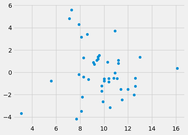
Now we want to see if we can predict these residuals with the Hemoglobin
values. Let’s use these residuals as our new y values, and fit a predicting
line using Hemoglobin.
First plot the residuals (y) against the Hemoglobin (x):
plt.scatter(ckdp['Hemoglobin'], residuals)
<matplotlib.collections.PathCollection at 0x7f25c457e590>
Then fit a line:
min_rmse_hgb = minimize(rmse_any_line,
                        initial_guess,
                        args=(ckdp['Hemoglobin'], residuals),
                        method='powell')
min_rmse_hgb
 message: Optimization terminated successfully.
 success: True
  status: 0
     fun: 2.221655830951226
       x: [-2.462e-06 -2.960e-03]
     nit: 1
   direc: [[ 1.000e+00  0.000e+00]
           [ 0.000e+00  1.000e+00]]
    nfev: 21
The results from minimize show that the line relating Hemoglobin and the
residuals has a negative slope, as we would expect; more severe kidney disease
leads to lower hemoglobin and higher creatinine. The root mean square error
has hardly changed, suggesting that Hemoglobin does not predict much, once we
have allowed for the predictions using Urea.
Multiple regression in one go#
Here we build the machinery as we did in the multiple regression page.
In particular, we are going to find three parameters:
An intercept;
A slope for the line relating
UreatoCreatinine;A slope for the line relating
HemoglobintoCreatinine.
In the multiple regression page, we found our best-fit slopes using the training set, but here we will use the whole dataset.
The multiple regression page did not allow for an intercept. Here we do allow for an intercept.
Otherwise, you will recognize much of this machinery from the multiple regression page.
def predict(intercept, slopes, row):
    """ Predict a value given an intercept, slopes and corresponding row values
    """
    return intercept + np.sum(slopes * np.array(row))
def rmse(intercept, slopes, attributes, y_values):
    """ Root mean square error for prediction of `y_values` from `attributes`

    Use `intercept` and `slopes` multiplied by `attributes` to give prediction.

    `attributes` is a data frame with numerical attributes to predict from.
    """
    errors = []
    for i in np.arange(len(y_values)):
        predicted = predict(intercept, slopes, attributes.iloc[i])
        actual = y_values.iloc[i]
        errors.append((actual - predicted) ** 2)
    return np.sqrt(np.mean(errors))
Here we calculate the root mean square error for an intercept of 1, and slopes
for Urea and Hemoglobin of 0 and 0.
rmse(1, [0, 0], ckdp.loc[:, 'Urea':], ckdp['Creatinine'])
6.28908245609285
def rmse_for_params(params, attributes, y_values):
    """ RMSE for intercept, slopes contained in `params`

    `params[0]` is the intercept.  `params[1:]` are the slopes.
    """
    intercept = params[0]
    slopes = params[1:]
    return rmse(intercept,
                slopes,
                attributes,
                y_values,
               )
Now we can get minimize to find the intercept and two slopes that minimize the root mean square error (and the sum of squared error):
attributes =  ckdp.loc[:, 'Urea':]
y_values = ckdp['Creatinine']
min_css = minimize(rmse_for_params, [0, 0, 0], method='powell',
                   args=(attributes, y_values))
min_css
 message: Optimization terminated successfully.
 success: True
  status: 0
     fun: 2.2155376442850536
       x: [ 1.025e+00  5.345e-02 -9.457e-02]
     nit: 6
   direc: [[ 1.000e+00  0.000e+00  0.000e+00]
           [ 4.412e-01  1.711e-02 -2.049e-01]
           [-5.009e+00  1.058e-02  3.779e-01]]
    nfev: 193
Just as for the simple regression case, and linregress, we can get our
parameters by calculation directly, in this case we were are using
least-squares as our criterion.
Don’t worry about the details of the function below. It contains the matrix
calculation to give us the same answer as minimize above, as long as we are
minimizing the root mean square error (or sum of squared error) for one or more
slopes and an intercept.
def multiple_regression_matrix(y_values, x_attributes):
    """ linregress equivalent for multiple slopes

    Parameters
    ----------
    y_values : array-like, shape (n,)
        Values to be predicted.
    x_attributes: array-like, shape (n, p)
        Something that can be made into a two-dimensional array (for example, an array or a data frame), that has ``n`` rows and `p` columns.

    Returns
    -------
    params : array, shape (p + 1,)
        Least-squares fit parameters, where first parameter is intercept value,
        and subsequent ``p`` parameters are slopes corresponding to ``p``
        columns in `x_attributes`.
    """
    intercept_col = np.ones(len(y_values))
    X = np.column_stack([intercept_col, x_attributes])
    return np.linalg.pinv(X) @ y_values
This function gives the same result as we got from minimize.
params = multiple_regression_matrix(y_values, attributes)
params
array([ 1.02388056, 0.05345685, -0.09432084])
Finally, let’s see StatsModels in action, to do the same calculation.
Here we specify that we want to fit a linear model to Creatinine as a
function of Urea and as a function of Hemoglobin. This has the same
meaning as above; that we will simultaneously fit the intercept, Urea slope
and the Hemoglobin slope.
multi_model = smf.ols(formula="Creatinine ~ Urea + Hemoglobin", data=ckdp)
multi_fit = multi_model.fit()
multi_fit.summary()
| Dep. Variable: | Creatinine | R-squared: | 0.717 |
|---|---|---|---|
| Model: | OLS | Adj. R-squared: | 0.703 |
| Method: | Least Squares | F-statistic: | 50.70 |
| Date: | Wed, 05 Jun 2024 | Prob (F-statistic): | 1.08e-11 |
| Time: | 16:05:58 | Log-Likelihood: | -95.221 |
| No. Observations: | 43 | AIC: | 196.4 |
| Df Residuals: | 40 | BIC: | 201.7 |
| Df Model: | 2 | ||
| Covariance Type: | nonrobust |
| coef | std err | t | P>|t| | [0.025 | 0.975] | |
|---|---|---|---|---|---|---|
| Intercept | 1.0239 | 2.416 | 0.424 | 0.674 | -3.859 | 5.907 |
| Urea | 0.0535 | 0.007 | 8.049 | 0.000 | 0.040 | 0.067 |
| Hemoglobin | -0.0943 | 0.197 | -0.478 | 0.635 | -0.493 | 0.305 |
| Omnibus: | 1.746 | Durbin-Watson: | 1.246 |
|---|---|---|---|
| Prob(Omnibus): | 0.418 | Jarque-Bera (JB): | 1.326 |
| Skew: | 0.430 | Prob(JB): | 0.515 |
| Kurtosis: | 2.960 | Cond. No. | 851. |
Notes:
[1] Standard Errors assume that the covariance matrix of the errors is correctly specified.
Notice again that StatsModels is doing the same calculation as above, and
finding the same result as minimize.
Multiple regression in 3D#
It can be useful to use a 3D plot to show what is going on here. minimize
and the other methods are finding these three parameters simultaneously:
An intercept;
A slope for
UreaA slope for
Hemoglobin.
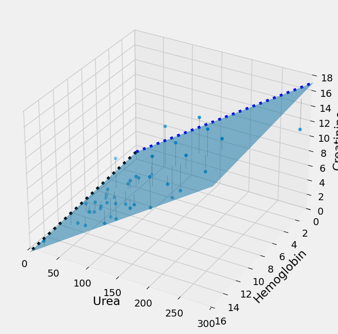
The plot below shows what this looks like, in 3D. Instead of the 2D case,
where we are fitting the y data values (Creatinine) with a single straight
line, here we are fitting the y data values with two straight lines. In 3D
these two straight lines form a plane, and we want the plane such that the sum
of squares of the distance of the y values from the plane (plotted) is as small
as possible. minimize will change the intercept and the two slopes to move
this plane around until it has minimized the error.
# Run this cell.
import mpl_toolkits.mplot3d  # (for Matplotlib < 3.2)
ax = plt.figure(figsize=(8,8)).add_subplot(111, projection='3d')
ax.scatter(ckdp['Urea'],
           ckdp['Hemoglobin'],
           ckdp['Creatinine']
          )
ax.set_xlabel('Urea')
ax.set_ylabel('Hemoglobin')
ax.set_zlabel('Creatinine')
intercept, urea_slope, hgb_slope = min_css.x
mx_urea, mx_hgb, mx_creat = 300, 16, 18
ax.plot([0, mx_urea],
        [intercept, intercept + urea_slope * mx_urea],
        0,
        zdir='y', color='blue', linestyle=':')
mx_hgb = ckdp['Hemoglobin'].max()
ax.plot([0, mx_hgb],
        [intercept, intercept + hgb_slope * mx_hgb],
        0,
        zdir='x', color='black', linestyle=':')
# Plot the fitting plane.
plane_x = np.linspace(0, mx_urea, 50)
plane_y = np.linspace(0, mx_hgb, 50)
X, Y = np.meshgrid(plane_x, plane_y)
Z = intercept + urea_slope * X + hgb_slope * Y
ax.plot_surface(X, Y, Z, alpha=0.5)
# Plot lines between each point and fitting plane
for i, row in ckdp.iterrows():
    x, y, actual = row['Urea'], row['Hemoglobin'], row['Creatinine']
    fitted = intercept + x * urea_slope + y * hgb_slope
    ax.plot([x, x], [y, y], [fitted, actual],
            linestyle=':',
            linewidth=0.5,
            color='black')
# Set the axis limits (and reverse y axis)
ax.set_xlim(0, mx_urea)
ax.set_ylim(mx_hgb, 0)
ax.set_zlim(0, mx_creat);