Multiple regression

Note

This page has content from the Multiple_Regression notebook of an older version of the UC Berkeley data science course. See the Berkeley course section of the license file.

Show code cell content Hide code cell content

import numpy as np
# Make random number generator.
rng = np.random.default_rng()
import pandas as pd
# Safe setting for Pandas.  Needs Pandas version >= 1.5.
pd.set_option('mode.copy_on_write', True)

import matplotlib.pyplot as plt
plt.style.use('fivethirtyeight')

np.set_printoptions(suppress=True)

Show code cell content Hide code cell content

def standard_units(any_numbers):
    "Convert any array of numbers to standard units."
    return (any_numbers - np.mean(any_numbers))/np.std(any_numbers)

def correlation(t, x, y):
    return np.mean(standard_units(t[x]) * standard_units(t[y]))

Now that we have explored ways to use multiple attributes to predict a categorical variable, let us return to predicting a quantitative variable. Predicting a numerical quantity is called regression, and a commonly used method to use multiple attributes for regression is called multiple linear regression.

Home Prices

The following dataset of house prices and attributes was collected over several years for the city of Ames, Iowa. A description of the dataset appears online. We will focus only a subset of the columns. We will try to predict the sale price column from the other columns.

all_sales = pd.read_csv('house.csv')
sales = all_sales.loc[np.logical_and(all_sales['Bldg Type'] == '1Fam',
                      all_sales['Sale Condition'] == 'Normal'),
    ['SalePrice', '1st Flr SF', '2nd Flr SF',
     'Total Bsmt SF', 'Garage Area',
     'Wood Deck SF', 'Open Porch SF', 'Lot Area',
     'Year Built', 'Yr Sold']]
sales.sort_values('SalePrice')

	SalePrice	1st Flr SF	2nd Flr SF	Total Bsmt SF	Garage Area	Wood Deck SF	Open Porch SF	Lot Area	Year Built	Yr Sold
2843	35000	498	0	498.0	216.0	0	0	8088	1922	2006
1901	39300	334	0	0.0	0.0	0	0	5000	1946	2007
1555	40000	649	668	649.0	250.0	0	54	8500	1920	2008
708	45000	612	0	0.0	308.0	0	0	5925	1940	2009
1220	52000	729	0	270.0	0.0	0	0	4130	1935	2008
...	...	...	...	...	...	...	...	...	...	...
2450	584500	1933	1567	1733.0	959.0	870	86	17242	1993	2006
432	610000	2674	0	2630.0	762.0	360	50	13693	2007	2009
1063	615000	2470	0	2535.0	789.0	154	65	12720	2003	2008
2445	625000	1831	1796	1930.0	807.0	361	76	35760	1995	2006
1767	755000	2444	1872	2444.0	832.0	382	50	21535	1994	2007

2002 rows × 10 columns

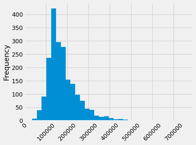
A histogram of sale prices shows a large amount of variability and a distribution that is clearly not normal. A long tail to the right contains a few houses that had very high prices. The short left tail does not contain any houses that sold for less than $35,000.

sales['SalePrice'].plot.hist(bins=32)
plt.xticks(rotation=45);

Correlation

No single attribute is sufficient to predict the sale price. For example, the area of first floor, measured in square feet, correlates with sale price but only explains some of its variability.

sales.plot.scatter('1st Flr SF', 'SalePrice')

<Axes: xlabel='1st Flr SF', ylabel='SalePrice'>

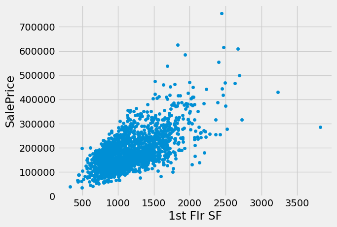
correlation(sales, 'SalePrice', '1st Flr SF')

0.6424662541030225

In fact, none of the individual attributes have a correlation with sale price that is above 0.7 (except for the sale price itself).

for col_name in sales.columns:
    r = correlation(sales, col_name, 'SalePrice')
    print(f'Correlation of {col_name} and SalePrice:\t{r:0.3f}', )

Correlation of SalePrice and SalePrice:	1.000
Correlation of 1st Flr SF and SalePrice:	0.642
Correlation of 2nd Flr SF and SalePrice:	0.358
Correlation of Total Bsmt SF and SalePrice:	0.653
Correlation of Garage Area and SalePrice:	0.639
Correlation of Wood Deck SF and SalePrice:	0.353
Correlation of Open Porch SF and SalePrice:	0.337
Correlation of Lot Area and SalePrice:	0.291
Correlation of Year Built and SalePrice:	0.565
Correlation of Yr Sold and SalePrice:	0.026

However, combining attributes can provide higher correlation. In particular, if we sum the first floor and second floor areas, the result has a higher correlation than any single attribute alone.

with_both = sales.copy()
with_both['Both Floors'] = sales['1st Flr SF'] + sales['2nd Flr SF']
correlation(with_both, 'SalePrice', 'Both Floors')

0.7821920556134877

This high correlation indicates that we should try to use more than one attribute to predict the sale price. In a dataset with multiple observed attributes and a single numerical value to be predicted (the sale price in this case), multiple linear regression can be an effective technique.

Multiple Linear Regression

In multiple linear regression, a numerical output is predicted from numerical input attributes by multiplying each attribute value by a different slope, then summing the results. In this example, the slope for the 1st Flr SF would represent the dollars per square foot of area on the first floor of the house that should be used in our prediction.

Before we begin prediction, we split our data randomly into a training and test set of equal size.

N = len(sales)
half_N = int(N / 2)
# Shuffle data frame by taking random sample with same number of rows.
shuffled_sales = sales.sample(n=N, replace=False)
train = shuffled_sales.iloc[:half_N]
test = shuffled_sales.iloc[half_N:]
print(len(train), 'training and', len(test), 'test instances.')

1001 training and 1001 test instances.

The slopes in multiple regression is an array that has one slope value for each attribute in an example. Predicting the sale price involves multiplying each attribute by the slope and summing the result.

def predict(slopes, row):
    return np.sum(slopes * np.array(row))

example_row = test.drop(columns='SalePrice').iloc[0]
print('Predicting sale price for:', example_row)
example_slopes = rng.normal(10, 1, len(example_row))
print('Using slopes:', example_slopes)
print('Result:', predict(example_slopes, example_row))

Predicting sale price for: 1st Flr SF        755.0
2nd Flr SF        755.0
Total Bsmt SF     755.0
Garage Area       296.0
Wood Deck SF      120.0
Open Porch SF       0.0
Lot Area         9084.0
Year Built       1940.0
Yr Sold          2009.0
Name: 798, dtype: float64
Using slopes: [12.18087627 11.17483824  9.65759708  9.61231848 10.93460662  9.48169596
  8.66900641  9.02314454  9.99560882]
Result: 145417.78204181476

The result is an estimated sale price, which can be compared to the actual sale price to assess whether the slopes provide accurate predictions. Since the example_slopes above were chosen at random, we should not expect them to provide accurate predictions at all.

print('Actual sale price:', test['SalePrice'].iloc[0])
print('Predicted sale price using random slopes:', predict(example_slopes, example_row))

Actual sale price: 108000
Predicted sale price using random slopes: 145417.78204181476

Least Squares Regression

The next step in performing multiple regression is to define the least squares objective. We perform the prediction for each row in the training set, and then compute the root mean squared error (RMSE) of the predictions from the actual prices.

train_prices = train['SalePrice']
train_attributes = train.drop(columns='SalePrice')

def rmse(slopes, attributes, y_values):
    errors = []
    for i in np.arange(len(y_values)):
        predicted = predict(slopes, attributes.iloc[i])
        actual = y_values.iloc[i]
        errors.append((actual - predicted) ** 2)
    return np.sqrt(np.mean(errors))

def rmse_train(slopes):
    return rmse(slopes, train_attributes, train_prices)

print('RMSE of all training examples using random slopes:', rmse_train(example_slopes))

RMSE of all training examples using random slopes: 67061.38443613885

Actually, the rmse routine above is correct, but it is slow, because we are looping through each rows in the data frame. Here’s a version that does the same calculation, but more efficiently, without a loop, using Numpy arrays. Don’t worry about the details, unless you are interested.

def rmse_fast(slopes, attributes, y_values):
    # Make an n by s array of slopes by copying the s slopes array n times.
    slopes_array = np.tile(slopes, [len(y_values), 1])
    # Multiply the n by s array by the corresponding attributes.
    predicted = np.sum(slopes_array * attributes, axis=1)
    errors = y_values - predicted
    return np.sqrt(np.mean(errors ** 2))

def rmse_train_fast(slopes):
    return rmse_fast(slopes, train_attributes, train_prices)

print('Fast RMSE of all training examples using random slopes:',
      rmse_train_fast(example_slopes))

Fast RMSE of all training examples using random slopes: 67061.38443613886

Finally, we use the minimize function to find the slopes with the lowest RMSE. Computation of the best slopes may take several minutes.

from scipy.optimize import minimize

We specify that we want to use the Powell method to search for the minimum.

# Use minimize to calculate smallest RMSE slopes.
multi_res = minimize(rmse_train_fast, example_slopes, method='powell')
multi_res

 message: Optimization terminated successfully.
 success: True
  status: 0
     fun: 34294.16768513197
       x: [ 7.718e+01  7.903e+01  6.126e+01  7.516e+01  4.367e+01
            2.988e+01  8.249e-01 -5.265e+00 -1.887e+01]
     nit: 15
   direc: [[ 1.643e+00 -6.513e-01 ... -1.031e+00 -1.864e+00]
           [ 0.000e+00  1.000e+00 ...  0.000e+00  0.000e+00]
           ...
           [-2.466e+00 -1.214e+01 ... -1.154e+01  3.666e-01]
           [-1.196e+00  9.645e-01 ... -3.675e-01 -3.062e-02]]
    nfev: 1231

best_slopes = multi_res.x
print('The best slopes for the training set:')
print('RMSE of all training examples using the best slopes:', rmse_train(best_slopes))
pd.DataFrame(data=[best_slopes], columns=train_attributes.columns)

The best slopes for the training set:
RMSE of all training examples using the best slopes: 34294.16768513198

	1st Flr SF	2nd Flr SF	Total Bsmt SF	Garage Area	Wood Deck SF	Open Porch SF	Lot Area	Year Built	Yr Sold
0	77.18376	79.030858	61.260786	75.158764	43.674909	29.878584	0.824891	-5.265169	-18.867835

Interpreting Multiple Regression

Let’s interpret these results. The best slopes give us a method for estimating the price of a house from its attributes. A square foot of area on the first floor is worth about 80 USD (the first slope), while one on the second floor is worth about 75 USD (the second slope). The final negative value describes the market: prices in later years were lower on average.

The RMSE of around 30,000 USD means that our best linear prediction of the sale price based on all of the attributes is off by around 30,000 USD on the training set, on average. We find a similar error when predicting prices on the test set, which indicates that our prediction method will generalize to other samples from the same population.

test_prices = test['SalePrice']
test_attributes = test.drop(columns='SalePrice')

def rmse_test(slopes):
    return rmse(slopes, test_attributes, test_prices)

rmse_linear = rmse_test(best_slopes)
print('Test set RMSE for multiple linear regression:', rmse_linear)

Test set RMSE for multiple linear regression: 33335.51769218093

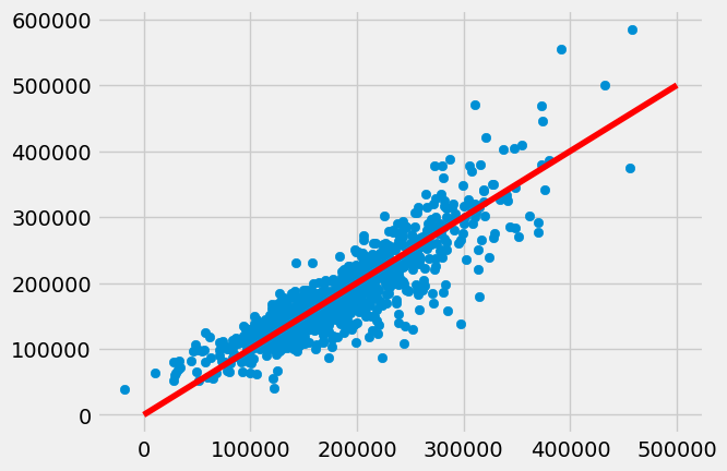
If the predictions were perfect, then a scatter plot of the predicted and actual values would be a straight line with slope 1. We see that most dots fall near that line, but there is some error in the predictions.

def fit(row):
    return sum(best_slopes * np.array(row))

fitted = test_attributes.apply(fit, axis=1)
plt.scatter(fitted, test_prices)
# Plot x=y line.
plt.plot([0, 5e5], [0, 5e5], color='red');

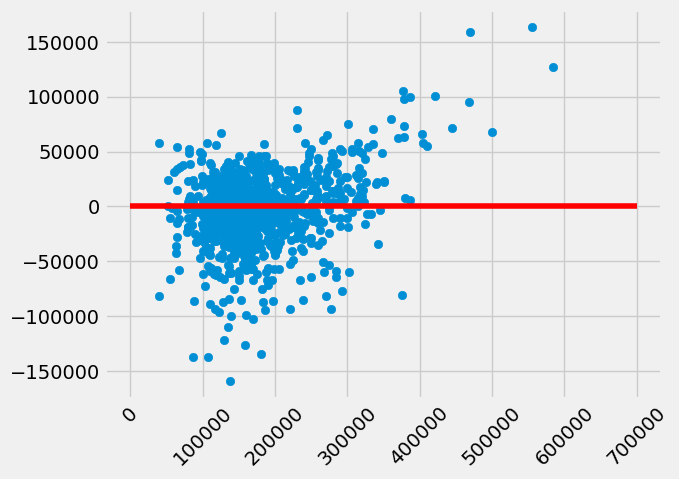
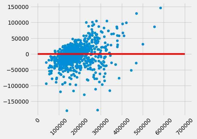
A residual plot for multiple regression typically compares the errors (residuals) to the actual values of the predicted variable. We see in the residual plot below that we have systematically underestimated the value of expensive houses, shown by the many positive residual values on the right side of the graph.

plt.scatter(test_prices, test_prices - fitted)
plt.plot([0, 7e5], [0, 0], color='red')
plt.xticks(rotation=45);

As with simple linear regression, interpreting the result of a predictor is at least as important as making predictions. There are many lessons about interpreting multiple regression that are not included in this textbook. A natural next step after completing this text would be to study linear modeling and regression in further depth.

Nearest Neighbors for Regression

Another approach to predicting the sale price of a house is to use the price of similar houses. This nearest neighbor approach is very similar to our classifier. To speed up computation, we will only use the attributes that had the highest correlation with the sale price in our original analysis.

train_nn = train.iloc[:, [0, 1, 2, 3, 4, 8]]
test_nn = test.iloc[:, [0, 1, 2, 3, 4, 8]]
train_nn.head(3)

	SalePrice	1st Flr SF	2nd Flr SF	Total Bsmt SF	Garage Area	Year Built
129	116500	858	0	858.0	0.0	1958
1397	144000	904	0	864.0	912.0	1970
2527	250000	1512	1142	1054.0	619.0	1968

The computation of closest neighbors is identical to a nearest-neighbor classifier. In this case, we will exclude the 'SalePrice' rather than the 'Class' column from the distance computation. The five nearest neighbors of the first test row are shown below.

def distance(pt1, pt2):
    """The distance between two points, represented as arrays."""
    return np.sqrt(sum((pt1 - pt2) ** 2))

def row_distance(row1, row2):
    """The distance between two rows of a table."""
    return distance(np.array(row1), np.array(row2))

def distances(training, example, output):
    """Compute the distance from example for each row in training."""
    attributes = training.drop(columns=output)

    def distance_from_example(row):
        return row_distance(row, example)

    out = training.copy()
    out['Distance'] = attributes.apply(distance_from_example, axis=1)
    return out

def closest(training, example, k, output):
    """Return a table of the k closest neighbors to example."""
    dist_df = distances(training, example, output)
    return dist_df.sort_values('Distance').head(k)

example_nn_row = test_nn.drop(columns='SalePrice').iloc[0]
closest(train_nn, example_nn_row, 5, 'SalePrice')

	SalePrice	1st Flr SF	2nd Flr SF	Total Bsmt SF	Garage Area	Year Built	Distance
1290	139500	728	728	728.0	308.0	1915	54.369109
2851	149000	755	755	755.0	216.0	1920	82.462113
1370	135000	756	713	756.0	216.0	1906	96.550505
282	113000	798	689	735.0	220.0	1945	111.382225
260	161750	689	703	689.0	299.0	1977	113.110565

One simple method for predicting the price is to average the prices of the nearest neighbors.

def predict_nn(example):
    """Return average of the price across the 5 nearest neighbors.
    """
    five_nearest = closest(train_nn, example, 5, 'SalePrice')
    return np.mean(five_nearest['SalePrice'])

predict_nn(example_nn_row)

139650.0

Finally, we can inspect whether our prediction is close to the true sale price for our one test example. Looks reasonable!

print('Actual sale price:', test_nn['SalePrice'].iloc[0])
print('Predicted sale price using nearest neighbors:', predict_nn(example_nn_row))

Actual sale price: 108000
Predicted sale price using nearest neighbors: 139650.0

Evaluation

To evaluate the performance of this approach for the whole test set, we apply predict_nn to each test example, then compute the root mean squared error of the predictions. Computation of the predictions may take several minutes.

attributes = test_nn.drop(columns='SalePrice')
nn_test_predictions = attributes.apply(predict_nn, axis=1)
rmse_nn = np.sqrt(np.mean((test_prices - nn_test_predictions) ** 2))

print('Test set RMSE for multiple linear regression: ', rmse_linear)
print('Test set RMSE for nearest neighbor regression:', rmse_nn)

Test set RMSE for multiple linear regression:  33335.51769218093
Test set RMSE for nearest neighbor regression: 32547.960557128175

For these data, the errors of the two techniques are quite similar! For different data sets, one technique might outperform another. By computing the RMSE of both techniques on the same data, we can compare methods fairly. One note of caution: the difference in performance might not be due to the technique at all; it might be due to the random variation due to sampling the training and test sets in the first place.

Finally, we can draw a residual plot for these predictions. We still underestimate the prices of the most expensive houses, but the bias does not appear to be as systematic. However, fewer residuals are very close to zero, indicating that fewer prices were predicted with very high accuracy.

plt.scatter(test_prices, test_prices - nn_test_predictions)
plt.plot([0, 7e5], [0, 0], color='red')
plt.xticks(rotation=45);

Note

This page has content from the Multiple_Regression notebook of an older version of the UC Berkeley data science course. See the Berkeley course section of the license file.