Sorting, heads and tails

# Load the Pandas data science library, call it 'pd'
import pandas as pd
# Turn on a setting to use Pandas more safely.
# We will discuss this setting later.
pd.set_option('mode.copy_on_write', True)

# Load the library for plotting, name it 'plt'
import matplotlib.pyplot as plt
# Make plots look a little more fancy
plt.style.use('fivethirtyeight')

In basic column indexing we found the slightly odd result that, for rich countries, there is little relationship between GDP and maternal mortality.

Here we investigate further, by looking at rich and poor countries separately.

In order to do that, we are going to sort our DataFrame using the .sort_values method, and the select the first and last group of rows, using the .head and .tail methods.

First let us return to the slightly processed DataFrame we were working on before:

# Original data frame before dropping missing values.
gender_data = pd.read_csv('gender_stats_min.csv')
gender_data_no_na = gender_data.dropna()
labeled_gdata = gender_data_no_na.set_index('country_code')
labeled_gdata

	country_name	gdp_us_billion	mat_mort_ratio	population
country_code
AFG	Afghanistan	19.961015	444.00	32.715838
AGO	Angola	111.936542	501.25	26.937545
ALB	Albania	12.327586	29.25	2.888280
ARE	United Arab Emirates	375.027082	6.00	9.080299
ARG	Argentina	550.980968	53.75	42.976675
...	...	...	...	...
WSM	Samoa	0.799887	54.75	0.192225
YEM	Yemen, Rep.	36.819337	399.75	26.246608
ZAF	South Africa	345.209888	143.75	54.177209
ZMB	Zambia	24.280990	233.75	15.633220
ZWE	Zimbabwe	15.495514	398.00	15.420964

179 rows × 4 columns

Here is the plot we saw before, with the unconvincing relationship of GDP to Maternal Mortality Rate (MMR).

plt.scatter(labeled_gdata['gdp_us_billion'],
            labeled_gdata['mat_mort_ratio'])
plt.title('MMR as a function of GDP')

Text(0.5, 1.0, 'MMR as a function of GDP')

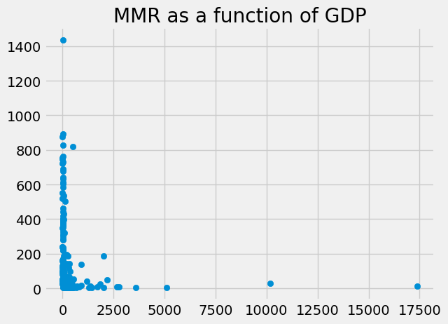
We wondered whether the relationship of GDP and MMR might be different for rich and poor countries.

To look at that, we can sort the DataFrame by the GDP values.

In order to do that, we use the .sort_values method, passing the column name containing the values we want to sort by:

gdata_by_gdp = labeled_gdata.sort_values('gdp_us_billion')
gdata_by_gdp

	country_name	gdp_us_billion	mat_mort_ratio	population
country_code
KIR	Kiribati	0.177431	95.00	0.110482
STP	Sao Tome and Principe	0.314540	159.50	0.191333
FSM	Micronesia, Fed. Sts.	0.319321	103.25	0.104118
TON	Tonga	0.439179	129.25	0.105909
COM	Comoros	0.603919	349.50	0.759556
...	...	...	...	...
GBR	United Kingdom	2768.864417	9.25	64.641557
DEU	Germany	3601.226158	6.25	81.281645
JPN	Japan	5106.024760	5.75	127.297102
CHN	China	10182.790479	28.75	1364.446000
USA	United States	17369.124600	14.00	318.558175

179 rows × 4 columns

Notice that the .sort_values method returned a new data frame with the rows in ascending order of the values in the given column (here gdp_us_billion). We therefore have a DataFrame where the richest countries are first and the poorest last.

Ascending order is the default sort order, but you can ask for descending order by giving the ascending keyword argument a value of False, like this:

gdata_by_desc_gdp = labeled_gdata.sort_values('gdp_us_billion',
                                               ascending=False)
gdata_by_desc_gdp

	country_name	gdp_us_billion	mat_mort_ratio	population
country_code
USA	United States	17369.124600	14.00	318.558175
CHN	China	10182.790479	28.75	1364.446000
JPN	Japan	5106.024760	5.75	127.297102
DEU	Germany	3601.226158	6.25	81.281645
GBR	United Kingdom	2768.864417	9.25	64.641557
...	...	...	...	...
COM	Comoros	0.603919	349.50	0.759556
TON	Tonga	0.439179	129.25	0.105909
FSM	Micronesia, Fed. Sts.	0.319321	103.25	0.104118
STP	Sao Tome and Principe	0.314540	159.50	0.191333
KIR	Kiribati	0.177431	95.00	0.110482

179 rows × 4 columns

Notice that now the richest countries are first and the poorest last.

Let us go back to the poorest to richest sorted DataFrame, gdata_by_gdp. The DataFrame has a .head method that, by default, will select the first 5 rows of the DataFrame:

gdata_by_gdp.head()

	country_name	gdp_us_billion	mat_mort_ratio	population
country_code
KIR	Kiribati	0.177431	95.00	0.110482
STP	Sao Tome and Principe	0.314540	159.50	0.191333
FSM	Micronesia, Fed. Sts.	0.319321	103.25	0.104118
TON	Tonga	0.439179	129.25	0.105909
COM	Comoros	0.603919	349.50	0.759556

Notice that the result is a new DataFrame that only has 5 rows.

In fact we often use .head to show a small sample of the DataFrame, and you will see that use throughout the rest of the course.

You can also give .head a number of rows you want. For example to select the 125 poorest countries (in terms of GDP), you could use:

poorest_125 = gdata_by_gdp.head(125)
poorest_125

	country_name	gdp_us_billion	mat_mort_ratio	population
country_code
KIR	Kiribati	0.177431	95.00	0.110482
STP	Sao Tome and Principe	0.314540	159.50	0.191333
FSM	Micronesia, Fed. Sts.	0.319321	103.25	0.104118
TON	Tonga	0.439179	129.25	0.105909
COM	Comoros	0.603919	349.50	0.759556
...	...	...	...	...
AGO	Angola	111.936542	501.25	26.937545
HUN	Hungary	129.470864	16.25	9.868180
UKR	Ukraine	135.379275	24.25	45.302704
KWT	Kuwait	156.226123	4.00	3.752954
BGD	Bangladesh	174.545099	194.75	159.371214

125 rows × 4 columns

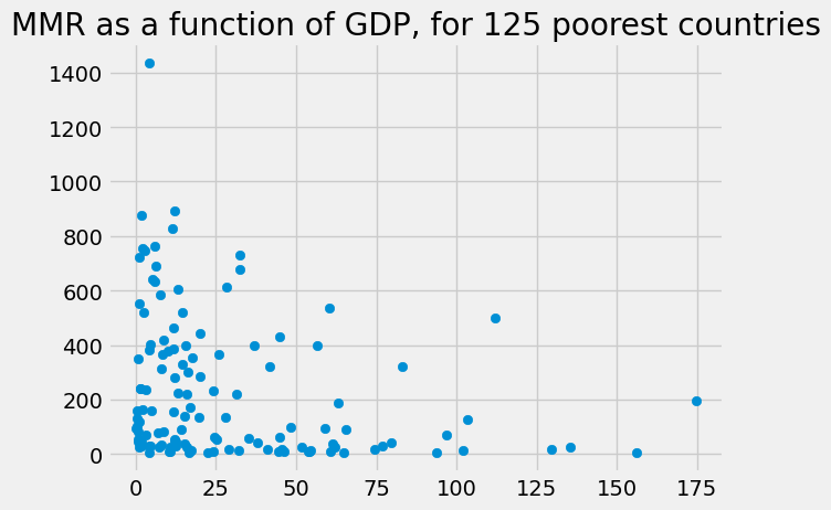
Now we have the rows corresponding to the 125 poorest countries, we can repeat our GDP / MMR plot, restricted to those countries:

plt.scatter(poorest_125['gdp_us_billion'], poorest_125['mat_mort_ratio'])
plt.title('MMR as a function of GDP, for 125 poorest countries')

Text(0.5, 1.0, 'MMR as a function of GDP, for 125 poorest countries')

If we sort the new DataFrame by the MMR values, we can see which of these 125 poorest countries are doing particularly well or badly in terms of MMR:

poorest_125.sort_values('mat_mort_ratio')

	country_name	gdp_us_billion	mat_mort_ratio	population
country_code
ISL	Iceland	16.741585	3.50	0.327387
BLR	Belarus	64.782942	4.00	9.480348
KWT	Kuwait	156.226123	4.00	3.752954
SVK	Slovak Republic	93.894473	6.00	5.418425
CYP	Cyprus	22.347398	7.00	1.152475
...	...	...	...	...
SOM	Somalia	5.785250	762.75	13.527075
SSD	South Sudan	11.480939	827.50	11.527917
CAF	Central African Republic	1.749110	875.75	4.529236
TCD	Chad	11.945942	892.25	13.574024
SLE	Sierra Leone	4.331604	1435.00	7.080112

125 rows × 4 columns

DataFrames also have .tail method that, by default, gives the last 5 rows of the DataFrame. For example, these are the 5 richest countries:

gdata_by_gdp.tail()

	country_name	gdp_us_billion	mat_mort_ratio	population
country_code
GBR	United Kingdom	2768.864417	9.25	64.641557
DEU	Germany	3601.226158	6.25	81.281645
JPN	Japan	5106.024760	5.75	127.297102
CHN	China	10182.790479	28.75	1364.446000
USA	United States	17369.124600	14.00	318.558175

Like .head we can give .tail a number of rows we want. Here we are looking at the last 25 rows of the sorted DataFrame, and therefore, the 25 richest countries:

richest_25 = gdata_by_gdp.tail(25)
richest_25

	country_name	gdp_us_billion	mat_mort_ratio	population
country_code
NGA	Nigeria	486.113579	818.50	176.551695
BEL	Belgium	494.221836	7.00	11.228495
POL	Poland	503.311262	3.00	38.009905
SWE	Sweden	540.626904	4.00	9.703634
ARG	Argentina	550.980968	53.75	42.976675
CHE	Switzerland	676.642359	5.25	8.185870
SAU	Saudi Arabia	707.936120	12.25	30.728077
NLD	Netherlands	819.285000	7.00	16.876547
TUR	Turkey	895.175577	17.50	77.034345
IDN	Indonesia	902.944866	136.75	255.064836
MEX	Mexico	1188.802780	40.00	124.203450
ESP	Spain	1299.724261	5.00	46.553128
KOR	Korea, Rep.	1346.751162	12.00	50.727212
AUS	Australia	1422.994116	6.00	23.444560
CAN	Canada	1708.473627	7.25	35.517119
RUS	Russian Federation	1822.691700	25.25	143.793504
ITA	Italy	2005.983980	4.00	60.378795
IND	India	2019.005411	185.25	1293.742537
BRA	Brazil	2198.765606	49.50	204.159544
FRA	France	2647.649725	8.75	66.302099
GBR	United Kingdom	2768.864417	9.25	64.641557
DEU	Germany	3601.226158	6.25	81.281645
JPN	Japan	5106.024760	5.75	127.297102
CHN	China	10182.790479	28.75	1364.446000
USA	United States	17369.124600	14.00	318.558175

plt.scatter(richest_25['gdp_us_billion'], richest_25['mat_mort_ratio'])
plt.title('MMR as a function of GDP, for 25 richest countries')

Text(0.5, 1.0, 'MMR as a function of GDP, for 25 richest countries')

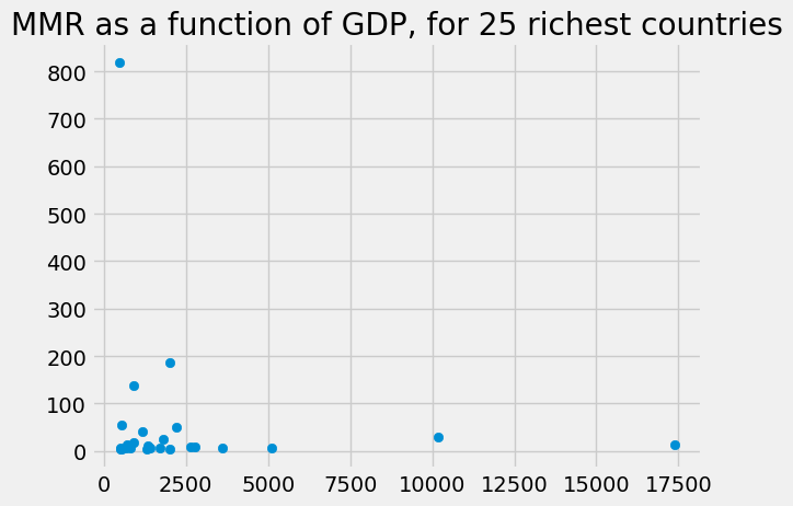
Again, we can sort by the MMR values to show the best and worst countries in terms of maternal health:

richest_25.sort_values('mat_mort_ratio')

	country_name	gdp_us_billion	mat_mort_ratio	population
country_code
POL	Poland	503.311262	3.00	38.009905
SWE	Sweden	540.626904	4.00	9.703634
ITA	Italy	2005.983980	4.00	60.378795
ESP	Spain	1299.724261	5.00	46.553128
CHE	Switzerland	676.642359	5.25	8.185870
JPN	Japan	5106.024760	5.75	127.297102
AUS	Australia	1422.994116	6.00	23.444560
DEU	Germany	3601.226158	6.25	81.281645
BEL	Belgium	494.221836	7.00	11.228495
NLD	Netherlands	819.285000	7.00	16.876547
CAN	Canada	1708.473627	7.25	35.517119
FRA	France	2647.649725	8.75	66.302099
GBR	United Kingdom	2768.864417	9.25	64.641557
KOR	Korea, Rep.	1346.751162	12.00	50.727212
SAU	Saudi Arabia	707.936120	12.25	30.728077
USA	United States	17369.124600	14.00	318.558175
TUR	Turkey	895.175577	17.50	77.034345
RUS	Russian Federation	1822.691700	25.25	143.793504
CHN	China	10182.790479	28.75	1364.446000
MEX	Mexico	1188.802780	40.00	124.203450
BRA	Brazil	2198.765606	49.50	204.159544
ARG	Argentina	550.980968	53.75	42.976675
IDN	Indonesia	902.944866	136.75	255.064836
IND	India	2019.005411	185.25	1293.742537
NGA	Nigeria	486.113579	818.50	176.551695

To investigate further, we need to do some calculations to adjust for the population.