The law of large numbers

Show code cell content Hide code cell content

# Don't change this cell; just run it.
import numpy as np
# Make random number generator.
rng = np.random.default_rng()
import matplotlib.pyplot as plt
# Make the plots look more fancy.
plt.style.use('fivethirtyeight')

You have already seen the law of large numbers in action, in the central limit theorem page.

The law of large numbers says that, as you take larger and larger samples from a population, the value of some statistic (such as the mean) from the sample will get closer and closer to the same statistic calculated from the population.

In this page, we look at probabilities and proportions.

Consider the set up in the Laws of Probability page. In that set up, we had a car park with 100 cars, of which 30 were red.

p_red = 30 / 100

Now let’s consider another variant. Now we have a huge car park. Let’s say we consider the largest car park in the world, with 20,000 spaces, in West Edmonton Mall, Edmonton, Alberta.

Again, we assume that there is an equal likelihood of any one car in the car park leaving next.

This time though, pretend we don’t know the proportion of red cars. We want to estimate that proportion by looking at a sample of cars leaving the car park.

In fact — although we don’t know this (wink) — the actual proportion in the full 20,000 car park is 30%

p_red = 0.3
p_not_red = 0.7

The car park is huge. We are going to take samples of around 100 or 1000 cars. Let’s assume that the car park is so big, that even after taking a sample of 999 cars, the probability for the next car being red or not red is the same (it won’t be, exactly, but near enough). So, we’ll draw our samples of cars with replacement, just to make things easier to think about, as if the car had gone out, entered our sample, and gone back in again, to become one of the 20,000 cars that can be next in our sample.

Here we think about what happens as we take samples with larger and larger number of cars, and take the proportion (this is also an average) of reds in the sample.

The law of large numbers says that, as we take more samples of the cars, the proportion of reds in the sample will get closer and closer to the probability of getting red on any one trial.

Let’s start by taking samples of 100 cars. One sample will be one trial.

Here’s one trial, taking 100 cars:

cars = rng.choice(['red', 'not_red'],
                   p=[p_red, p_not_red],
                   size=100)
prop = np.count_nonzero(cars == 'red') / 100
print('Proportion of red', prop)

Proportion of red 0.31

Now we run 1000 trials. On each trial we get 100 cars, and record the proportion of red. Finally we show the spread of proportions that we get.

n_iters = 10000
n_cars = 100
props = np.zeros(n_iters)
for i in np.arange(n_iters):
    samples = rng.choice(['red', 'not_red'],
                         p=[p_red, p_not_red],
                         size=n_cars)
    props[i] = np.count_nonzero(samples == 'red') / n_cars
# Define the bins for the histogram to make them comparable across n_cars
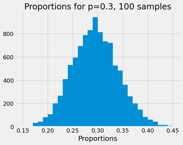
plt.hist(props, bins=np.arange(0.15, 0.45, 0.01))
plt.xlabel('Proportions')
plt.title('Proportions for p=0.3, ' +  str(n_cars) + ' samples');

Because we want to repeat this several times with different numbers of cars, we make the code above into a function:

def show_proportions(n_cars, n_iters=10000):
    props = np.zeros(n_iters)
    for i in np.arange(n_iters):
        samples = rng.choice(['red', 'not_red'],
                              p=[p_red, p_not_red],
                              size=n_cars)
        props[i] = np.count_nonzero(samples == 'red') / n_cars
    # Define the bins for the histogram to make them comparable across n_cars
    plt.hist(props, bins=np.arange(0.15, 0.45, 0.01))
    plt.xlabel('Proportions')
    plt.title('Proportions for p=0.3, ' +  str(n_cars) + ' samples');

Here is the spread (distribution) we saw above, for 100 car samples, but using the function.

show_proportions(100)

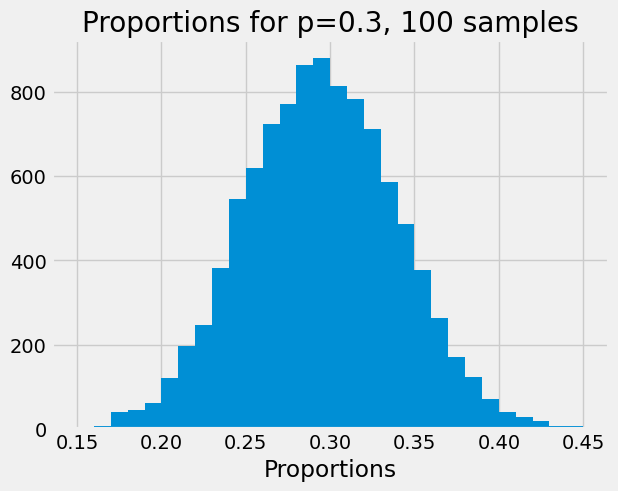
The law of large numbers says that, the larger the number of cars in our sample, the closer the proportions become, to the expected proportion — which is the probability, 0.3.

Here we increase the number of cars in the sample to 1000.

show_proportions(1000)

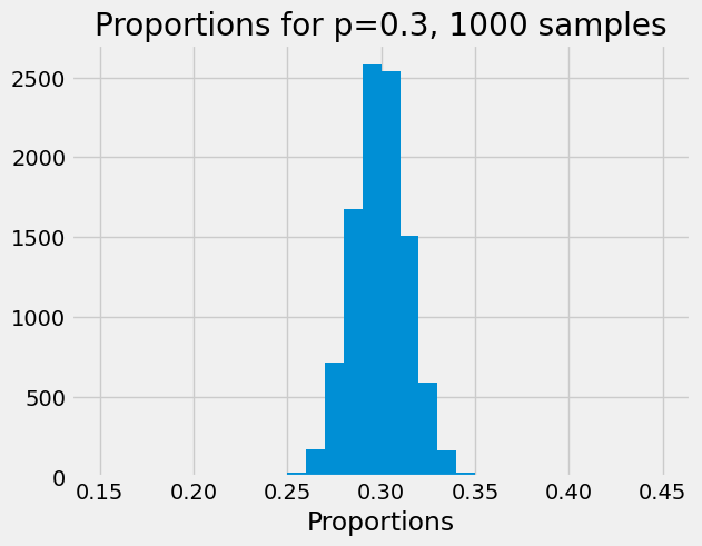
Notice that the distribution has got considerably tighter; the proportions do still vary from trial to trial, but they vary less than for the case with 100 cars, and they are, on average, a lot close to the expected value of 0.3.

Here is the result of trials taking proportions of 10000 cars:

show_proportions(10000)

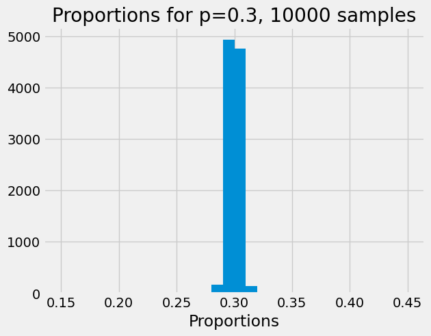
Now the distribution is getting very tight around the expected value.

In fact, the law of large numbers tells us that, as the number of cars in our sample gets very high, the proportion of red in the sample gets very close to 0.3.

Another way of saying this, is that in the long run, if we take huge numbers of cars in our sample, our proportions will get closer and closer to the probability on the single trial — of 0.3.

One useful way to think of this, is of each individual car in the sample flowing along one of two paths. There is a probability of 0.3 that the car will flow along the red path, and a probability of 0.7 that it will flow along the not_red path. In the long run, 30% of the cars end up at the end of the red path, and 70% of trials end up at the end of the not_red path.

These diagrams of flow can be called Sankey diagrams. They are useful for thinking about probability.