Series are like arrays

In this page, we look at Pandas’ Series. Series are the Pandas type that represents a column of data.

# Load the Numpy array library, call it 'np'
import numpy as np
# Load the Pandas data science library, call it 'pd'
import pandas as pd
# Turn on a setting to use Pandas more safely.
# We will discuss this setting later.
pd.set_option('mode.copy_on_write', True)

# Load the library for plotting, name it 'plt'
import matplotlib.pyplot as plt
# Make plots look a little more fancy
plt.style.use('fivethirtyeight')

We return to our original data frame, with the missing values dropped, and the rows labels with the country codes:

# Original data frame before dropping missing values.
gender_data = pd.read_csv('gender_stats_min.csv')
gender_data_no_na = gender_data.dropna()
labeled_gdata = gender_data_no_na.set_index('country_code')
labeled_gdata.head()

	country_name	gdp_us_billion	mat_mort_ratio	population
country_code
AFG	Afghanistan	19.961015	444.00	32.715838
AGO	Angola	111.936542	501.25	26.937545
ALB	Albania	12.327586	29.25	2.888280
ARE	United Arab Emirates	375.027082	6.00	9.080299
ARG	Argentina	550.980968	53.75	42.976675

We found that there was a rather unconvincing relationship between the GDP values, and the Maternal Mortality Rate (MMR) values.

First we fetch those values from their corresponding DataFrame columns, using direct indexing with column labels:

gdp = labeled_gdata['gdp_us_billion']
gdp

country_code
AFG     19.961015
AGO    111.936542
ALB     12.327586
ARE    375.027082
ARG    550.980968
          ...    
WSM      0.799887
YEM     36.819337
ZAF    345.209888
ZMB     24.280990
ZWE     15.495514
Name: gdp_us_billion, Length: 179, dtype: float64

mmr = labeled_gdata['mat_mort_ratio']
mmr

country_code
AFG    444.00
AGO    501.25
ALB     29.25
ARE      6.00
ARG     53.75
        ...  
WSM     54.75
YEM    399.75
ZAF    143.75
ZMB    233.75
ZWE    398.00
Name: mat_mort_ratio, Length: 179, dtype: float64

We plot the two Series against each other to remind ourselves of the relationship.

plt.scatter(gdp, mmr)
plt.title('Maternal mortality ratio as a function of GDP')

Text(0.5, 1.0, 'Maternal mortality ratio as a function of GDP')

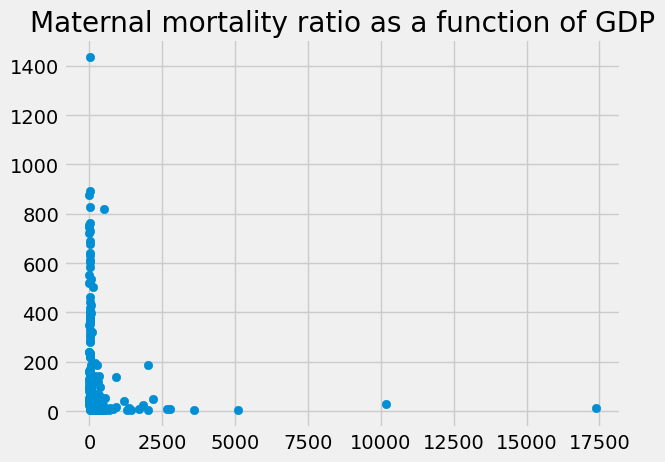
Our question was whether the GDP might be a misleading measure, because it will depend, in part, on the population. More people can earn more money. We were interested to calculate a GDP value adjusted for the population.

But first, let us investigate Series a little more.

Series have some of the same methods as DataFrames

gdp is a Series:

type(gdp)

pandas.core.series.Series

As the DdataFrame has .head and .tail methods to show the first 5 and last 5 rows (by default), so the Series has .head and .tail:

gdp.head()

country_code
AFG     19.961015
AGO    111.936542
ALB     12.327586
ARE    375.027082
ARG    550.980968
Name: gdp_us_billion, dtype: float64

gdp.head(10)

country_code
AFG      19.961015
AGO     111.936542
ALB      12.327586
ARE     375.027082
ARG     550.980968
ARM      10.885362
AUS    1422.994116
AUT     407.494276
AZE      62.003001
BDI       2.876978
Name: gdp_us_billion, dtype: float64

gdp.tail()

country_code
WSM      0.799887
YEM     36.819337
ZAF    345.209888
ZMB     24.280990
ZWE     15.495514
Name: gdp_us_billion, dtype: float64

As you remember we can sort a DataFrame using the .sort_values method:

labeled_gdata.sort_values('gdp_us_billion')

	country_name	gdp_us_billion	mat_mort_ratio	population
country_code
KIR	Kiribati	0.177431	95.00	0.110482
STP	Sao Tome and Principe	0.314540	159.50	0.191333
FSM	Micronesia, Fed. Sts.	0.319321	103.25	0.104118
TON	Tonga	0.439179	129.25	0.105909
COM	Comoros	0.603919	349.50	0.759556
...	...	...	...	...
GBR	United Kingdom	2768.864417	9.25	64.641557
DEU	Germany	3601.226158	6.25	81.281645
JPN	Japan	5106.024760	5.75	127.297102
CHN	China	10182.790479	28.75	1364.446000
USA	United States	17369.124600	14.00	318.558175

179 rows × 4 columns

This is also true of a Series:

gdp.sort_values()

country_code
KIR        0.177431
STP        0.314540
FSM        0.319321
TON        0.439179
COM        0.603919
           ...     
GBR     2768.864417
DEU     3601.226158
JPN     5106.024760
CHN    10182.790479
USA    17369.124600
Name: gdp_us_billion, Length: 179, dtype: float64

Notice that, for the Series, we don’t have to give .sort_values the column name, because the Series is already the column we want to sort.

A Series has values and labels

A Series is like an array, in that it contains a sequence of values. In fact, the Series holds that sequence of values in an array. You can get the sequence of values from the Series with the np.array function:

# The values from a Series as an array
np.array(gdp)

array([1.99610151e+01, 1.11936542e+02, 1.23275859e+01, 3.75027082e+02,
       5.50980968e+02, 1.08853625e+01, 1.42299412e+03, 4.07494276e+02,
       6.20030013e+01, 2.87697831e+00, 4.94221836e+02, 8.77815063e+00,
       1.17530544e+01, 1.74545099e+02, 5.37976122e+01, 3.20040106e+01,
       8.68800000e+00, 1.73233271e+01, 6.47829419e+01, 1.68032497e+00,
       3.15093236e+01, 2.19876561e+03, 4.41308000e+00, 1.57192226e+01,
       1.97514532e+00, 1.51133948e+01, 1.74910987e+00, 1.70847363e+03,
       6.76642359e+02, 2.59208554e+02, 1.01827905e+04, 3.25358753e+01,
       2.81421556e+01, 3.25386626e+01, 1.16655768e+01, 3.40405888e+02,
       6.03918965e-01, 1.73054354e+00, 5.18299661e+01, 7.95194750e+01,
       2.23473982e+01, 2.00535631e+02, 3.60122616e+03, 1.53090824e+00,
       3.26096204e+02, 6.54993582e+01, 1.90734615e+02, 9.66650964e+01,
       3.08496722e+02, 1.29972426e+03, 2.39872406e+01, 5.66819675e+01,
       2.53688521e+02, 4.33093138e+00, 2.64764973e+03, 3.19320780e-01,
       1.62834944e+01, 2.76886442e+03, 1.53644509e+01, 4.17188959e+01,
       6.30423092e+00, 9.13773107e-01, 1.06283063e+00, 1.76270598e+01,
       2.22206258e+02, 9.10843446e-01, 5.90985382e+01, 3.10872347e+00,
       1.98292083e+01, 5.40874424e+01, 8.37327626e+00, 1.29470864e+02,
       9.02944866e+02, 2.01900541e+03, 2.59826259e+02, 4.79398094e+02,
       2.07685388e+02, 1.67415845e+01, 2.95577073e+02, 2.00598398e+03,
       1.42531394e+01, 3.53060370e+01, 5.10602476e+03, 1.96818842e+02,
       6.02503997e+01, 6.92754607e+00, 1.68665072e+01, 1.77430636e-01,
       1.34675116e+03, 1.56226123e+02, 1.31391168e+01, 4.55819922e+01,
       1.96600000e+00, 1.36256387e+00, 7.68085057e+01, 2.45329837e+00,
       4.44015393e+01, 6.05560448e+01, 2.88860491e+01, 1.03402329e+02,
       7.30314452e+00, 1.01848586e+01, 3.08680306e+00, 1.18880278e+03,
       1.05752957e+01, 1.32103703e+01, 1.03510583e+01, 6.30938400e+01,
       4.26661171e+00, 1.20006207e+01, 1.46655026e+01, 5.16400962e+00,
       1.20895485e+01, 5.88343532e+00, 3.13686193e+02, 1.20684535e+01,
       7.50148231e+00, 4.86113579e+02, 1.18747997e+01, 8.19285000e+02,
       4.57585186e+02, 2.01166147e+01, 1.85598413e+02, 7.45575405e+01,
       2.50934589e+02, 4.82593427e+01, 1.95244387e+02, 2.80838449e+02,
       1.59111580e+01, 5.03311262e+02, 1.02107758e+02, 2.15143697e+02,
       2.78331214e+01, 1.25082200e+01, 1.81779231e+02, 1.85384091e+02,
       1.82269170e+03, 7.91832002e+00, 7.07936120e+02, 8.30167318e+01,
       1.45395548e+01, 2.98724394e+02, 1.11453462e+00, 4.33160391e+00,
       2.52137140e+01, 5.78525000e+00, 4.10756437e+01, 1.14809386e+01,
       3.14539986e-01, 4.77315902e+00, 9.38944735e+01, 4.60488627e+01,
       5.40626904e+02, 4.34681654e+00, 1.19459416e+01, 4.18361027e+00,
       4.06136904e+02, 8.03622825e+00, 3.79730958e+01, 1.36142965e+00,
       4.39178883e-01, 2.45709470e+01, 4.48243740e+01, 8.95175577e+02,
       4.49355418e+01, 2.59414607e+01, 1.35379275e+02, 5.43451323e+01,
       1.73691246e+04, 6.13406487e+01, 7.30106763e-01, 3.76146268e+02,
       1.81820736e+02, 7.82875953e-01, 7.99887347e-01, 3.68193365e+01,
       3.45209888e+02, 2.42809899e+01, 1.54955139e+01])

Notice that, by making the Series into an array, we have thrown away to the row labels.

The Series also has labels. These labels correspond to the row labels for the DataFrame, and, like them, you can find the Series labels in the Series .index attribute:

gdp.index

Index(['AFG', 'AGO', 'ALB', 'ARE', 'ARG', 'ARM', 'AUS', 'AUT', 'AZE', 'BDI',
       ...
       'UZB', 'VCT', 'VEN', 'VNM', 'VUT', 'WSM', 'YEM', 'ZAF', 'ZMB', 'ZWE'],
      dtype='object', name='country_code', length=179)

Think of the Series as the association of the values (np.array(gdp)) and the corresponding labels (gdp.index).

Calculations on Series work like calculation on arrays

As you remember, calculations on arrays work elementwise. For example, if you multiply an array by a number, that has the effect of making a new array, where the result is each element of the original array multiplied by the number.

The same is true of calculations on Series. For example, we might want to calculate the GDP in US million dollars instead of its current values in US billion:

# GDP in US million
gdp * 1000

country_code
AFG     19961.015094
AGO    111936.542134
ALB     12327.585927
ARE    375027.082337
ARG    550980.967906
           ...      
WSM       799.887347
YEM     36819.336505
ZAF    345209.888495
ZMB     24280.989920
ZWE     15495.513860
Name: gdp_us_billion, Length: 179, dtype: float64

The elementwise calculations also apply to operations on two Series. In fact, that is the key to solving our problem of getting the GDP values divided by the population. We make the population DataFrame column into a Series.

# Population is in millions.
pop = labeled_gdata['population']
pop

country_code
AFG    32.715838
AGO    26.937545
ALB     2.888280
ARE     9.080299
ARG    42.976675
         ...    
WSM     0.192225
YEM    26.246608
ZAF    54.177209
ZMB    15.633220
ZWE    15.420964
Name: population, Length: 179, dtype: float64

Then we can use elementwise calculation to divide the values in the two series, elementwise, like this:

# GDP per million people.
gdp_per_mcap = gdp / pop
gdp_per_mcap

country_code
AFG     0.610133
AGO     4.155410
ALB     4.268141
ARE    41.301180
ARG    12.820465
         ...    
WSM     4.161204
YEM     1.402823
ZAF     6.371865
ZMB     1.553166
ZWE     1.004834
Length: 179, dtype: float64

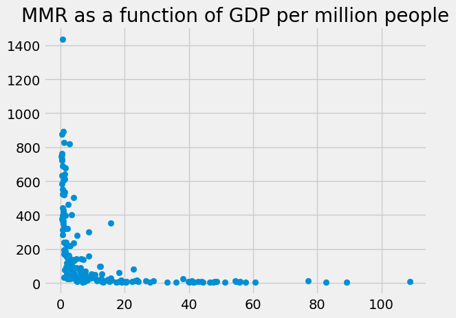
This is what we wanted, the GDP divided by the population. Let’s see if there is a more convincing relationship between the GDP per million and the MMR:

plt.scatter(gdp_per_mcap, mmr)
plt.title('MMR as a function of GDP per million people')

Text(0.5, 1.0, 'MMR as a function of GDP per million people')

You can insert Series as columns into DataFrames

Just as you can make a Series by indexing into a DataFrame, you can insert a Series into a DataFrame as a column, by using indexing.

# Insert new column into DataFrame
labeled_gdata['gdp_per_mcap'] = gdp_per_mcap
labeled_gdata.head()

	country_name	gdp_us_billion	mat_mort_ratio	population	gdp_per_mcap
country_code
AFG	Afghanistan	19.961015	444.00	32.715838	0.610133
AGO	Angola	111.936542	501.25	26.937545	4.155410
ALB	Albania	12.327586	29.25	2.888280	4.268141
ARE	United Arab Emirates	375.027082	6.00	9.080299	41.301180
ARG	Argentina	550.980968	53.75	42.976675	12.820465

Scroll across the DataFrame display to see the new column at the end.

Here we inserted the Series into the labeled_gdata DataFrame as new column, by using direct indexing with column label on the Right Hand Side. Read the assignment above as “make a column called ‘gdp_per_mcap’ in labeled_gdata and fill it with the values from the gdp_per_mcap Series”.

With the Series data in the DataFrame, we can sort the DataFrame by the new GDP per million values:

gdata_by_gdp_mcap = labeled_gdata.sort_values('gdp_per_mcap')
gdata_by_gdp_mcap.head()

	country_name	gdp_us_billion	mat_mort_ratio	population	gdp_per_mcap
country_code
BDI	Burundi	2.876978	747.25	9.907015	0.290398
MWI	Malawi	5.883435	633.00	17.081694	0.344429
CAF	Central African Republic	1.749110	875.75	4.529236	0.386182
NER	Niger	7.501482	585.50	19.175235	0.391207
SOM	Somalia	5.785250	762.75	13.527075	0.427679

Let us look to see if sorting this way gives a clearer picture of the relationship of income to MMR. Get the richest 25 countries in terms of GDP per million:

richest_per_mcap_25 = gdata_by_gdp_mcap.tail(25)
richest_per_mcap_25

	country_name	gdp_us_billion	mat_mort_ratio	population	gdp_per_mcap
country_code
ISR	Israel	295.577073	5.00	8.222580	35.946999
BRN	Brunei Darussalam	15.719223	23.75	0.411581	38.192275
FRA	France	2647.649725	8.75	66.302099	39.933121
JPN	Japan	5106.024760	5.75	127.297102	40.111084
NZL	New Zealand	185.598413	11.50	4.529660	40.974027
ARE	United Arab Emirates	375.027082	6.00	9.080299	41.301180
KWT	Kuwait	156.226123	4.00	3.752954	41.627510
GBR	United Kingdom	2768.864417	9.25	64.641557	42.834123
BEL	Belgium	494.221836	7.00	11.228495	44.014967
DEU	Germany	3601.226158	6.25	81.281645	44.305528
FIN	Finland	253.688521	3.00	5.457816	46.481688
AUT	Austria	407.494276	4.00	8.566294	47.569497
CAN	Canada	1708.473627	7.25	35.517119	48.102821
NLD	Netherlands	819.285000	7.00	16.876547	48.545773
ISL	Iceland	16.741585	3.50	0.327387	51.137049
USA	United States	17369.124600	14.00	318.558175	54.524184
SGP	Singapore	298.724394	10.75	5.464722	54.664156
SWE	Sweden	540.626904	4.00	9.703634	55.713859
IRL	Ireland	259.826259	8.00	4.650469	55.870977
DNK	Denmark	326.096204	6.75	5.652916	57.686370
AUS	Australia	1422.994116	6.00	23.444560	60.696133
QAT	Qatar	181.779231	13.25	2.357161	77.117881
CHE	Switzerland	676.642359	5.25	8.185870	82.659798
NOR	Norway	457.585186	5.00	5.131393	89.173681
LUX	Luxembourg	60.556045	10.25	0.556640	108.788486

Plot the relationship of GDP per million and MMR:

plt.scatter(richest_per_mcap_25['gdp_per_mcap'], richest_per_mcap_25['mat_mort_ratio'])
plt.title('MMR as function of GDP per million, richest 25')

Text(0.5, 1.0, 'MMR as function of GDP per million, richest 25')

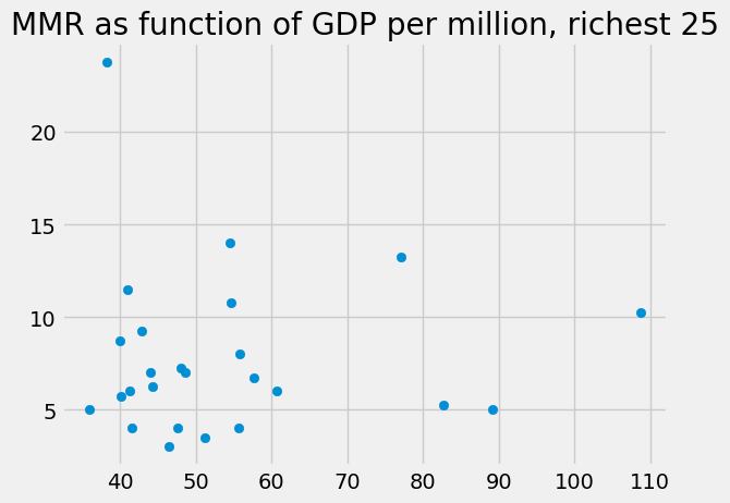
We might be interested in looking at the richest countries in terms of the MMR, by sorting. The countries doing best at reducing MMR are first, those doing worst are last.

richest_per_mcap_25.sort_values('mat_mort_ratio')

	country_name	gdp_us_billion	mat_mort_ratio	population	gdp_per_mcap
country_code
FIN	Finland	253.688521	3.00	5.457816	46.481688
ISL	Iceland	16.741585	3.50	0.327387	51.137049
KWT	Kuwait	156.226123	4.00	3.752954	41.627510
SWE	Sweden	540.626904	4.00	9.703634	55.713859
AUT	Austria	407.494276	4.00	8.566294	47.569497
ISR	Israel	295.577073	5.00	8.222580	35.946999
NOR	Norway	457.585186	5.00	5.131393	89.173681
CHE	Switzerland	676.642359	5.25	8.185870	82.659798
JPN	Japan	5106.024760	5.75	127.297102	40.111084
AUS	Australia	1422.994116	6.00	23.444560	60.696133
ARE	United Arab Emirates	375.027082	6.00	9.080299	41.301180
DEU	Germany	3601.226158	6.25	81.281645	44.305528
DNK	Denmark	326.096204	6.75	5.652916	57.686370
BEL	Belgium	494.221836	7.00	11.228495	44.014967
NLD	Netherlands	819.285000	7.00	16.876547	48.545773
CAN	Canada	1708.473627	7.25	35.517119	48.102821
IRL	Ireland	259.826259	8.00	4.650469	55.870977
FRA	France	2647.649725	8.75	66.302099	39.933121
GBR	United Kingdom	2768.864417	9.25	64.641557	42.834123
LUX	Luxembourg	60.556045	10.25	0.556640	108.788486
SGP	Singapore	298.724394	10.75	5.464722	54.664156
NZL	New Zealand	185.598413	11.50	4.529660	40.974027
QAT	Qatar	181.779231	13.25	2.357161	77.117881
USA	United States	17369.124600	14.00	318.558175	54.524184
BRN	Brunei Darussalam	15.719223	23.75	0.411581	38.192275

Conversely, we might want to take the poorest 75 by GDP per million, and look at the best and worst by MMR:

poorest_by_mcap_75 = gdata_by_gdp_mcap.head(75)
poorest_by_mcap_75.sort_values('mat_mort_ratio')

	country_name	gdp_us_billion	mat_mort_ratio	population	gdp_per_mcap
country_code
MDA	Moldova	7.303145	24.25	3.556118	2.053685
UKR	Ukraine	135.379275	24.25	45.302704	2.988327
ARM	Armenia	10.885362	27.25	2.904683	3.747521
LKA	Sri Lanka	76.808506	31.25	20.790000	3.694493
TJK	Tajikistan	8.036228	33.25	8.363844	0.960830
...	...	...	...	...	...
NGA	Nigeria	486.113579	818.50	176.551695	2.753378
SSD	South Sudan	11.480939	827.50	11.527917	0.995925
CAF	Central African Republic	1.749110	875.75	4.529236	0.386182
TCD	Chad	11.945942	892.25	13.574024	0.880059
SLE	Sierra Leone	4.331604	1435.00	7.080112	0.611799

75 rows × 5 columns