Sum of squares, root mean square

The mean and slopes page used the Sum of Squared Error (SSE) as the measure of how well a particular slope fits the data.

Here we will think about another, derived measure, called the Root Mean Square Error.

First, let us go back to the original problem.

Hemoglobin and Packed Cell Volume, again

# Run this cell.
import numpy as np
import matplotlib.pyplot as plt
# Make plots look a little bit more fancy
plt.style.use('fivethirtyeight')
# Print to 4 decimal places, show tiny values as 0
np.set_printoptions(precision=4, suppress=True)
import pandas as pd
pd.set_option('mode.copy_on_write', True)

We go back to the data on chronic kidney disease.

Download the data to your computer via this link: ckd_clean.csv.

We were interested to find the “best” slope for a line that relates the blood hemoglobin measures in each patient, with their corresponding Packed Cell Volume (PCV) blood measure:

# Run this cell
ckd = pd.read_csv('ckd_clean.csv')
hgb = np.array(ckd['Hemoglobin'])
pcv = np.array(ckd['Packed Cell Volume'])
# Plot HGB on the x axis, PCV on the y axis
plt.plot(hgb, pcv, 'o')
plt.xlabel('Hemoglobin concentration')
plt.ylabel('Packed cell volume')

Text(0, 0.5, 'Packed cell volume')

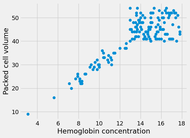
We are assuming our line goes through hgb == 0 and pcv == 0, on the basis that the red blood cells measured by PCV contain all the hemoglobin, so if PCV is 0 then hemoglobin must be 0 and vice versa. Our predicted values for PCV for each patient are the given by some slopes multiplied by the corresponding hemoglobin value for that patient.

For example, say the slope is 2.25, then the predicted PCV values are:

s = 2.25
predicted_pcv = s * hgb
predicted_pcv[:10]

array([25.2  , 21.375, 24.3  , 12.6  , 17.325, 22.05 , 28.125, 22.5  ,
       23.625, 22.05 ])

The errors for these predictions are:

errors = pcv - predicted_pcv
errors[:10]

array([6.8  , 7.625, 7.7  , 3.4  , 6.675, 9.95 , 8.875, 6.5  , 9.375,
       5.95 ])

Sum of Squared error

We decided to use the Sum of Squared Error (SSE) as a measure of the quality of fit.

The sum of squared error is nothing but:

sse = np.sum(errors ** 2)
sse

23274.978750000002

Here’s a function to return the SSE. We call this the cost function because it calculates a cost in terms of error for a given slope.

def calc_sse(slope):
    predicted_pcv = hgb * slope  # 'hgb' comes from the top level
    errors = pcv - predicted_pcv # 'pcv' comes from the top level
    return np.sum(errors ** 2)

# Recalculate SSE for slope of interest.
calc_sse(2.25)

23274.978750000002

Then we used minimize to find the slope that minimizes the SSE:

from scipy.optimize import minimize
# 2.25 below is the slope value to start the search.
res_sse = minimize(calc_sse, 2.25)
res_sse

  message: Desired error not necessarily achieved due to precision loss.
  success: False
   status: 2
      fun: 3619.6157878183285
        x: [ 3.047e+00]
      nit: 2
      jac: [ 1.221e-04]
 hess_inv: [[ 1.618e-05]]
     nfev: 70
     njev: 29

Notice the warning - there was some inaccuracy in the calculation. We may try slightly different cost functions to avoid that.

Root mean squared error

One problem with the SSE is that it can get very large, especially if there are a large number of points. When the values get large, this can cause calculation problems. Very large numbers for SSE can make it harder to think about the SSE values.

One way of allowing for the number of points, is to use the mean square error (MSE), instead of the SSE. Here is the MSE cost function.

def calc_mse(slope):
    predicted_pcv = hgb * slope  # 'hgb' comes from the top level
    errors = pcv - predicted_pcv # 'pcv' comes from the top level
    return np.mean(errors ** 2)  # Notice mean instead of sum

We try minimize again, to find the best slope.

# 2.25 below is the slope value to start the search.
res_mse = minimize(calc_mse, 2.25)
res_mse

  message: Optimization terminated successfully.
  success: True
   status: 0
      fun: 22.908960682394497
        x: [ 3.047e+00]
      nit: 2
      jac: [ 2.384e-07]
 hess_inv: [[ 2.556e-03]]
     nfev: 6
     njev: 3

Notice there is no warning this time in the optimization message.

Notice that running minimize on the MSE found the same slope as it did for the SSE. The resulting cost function fun value is the original SSE value divided by the number of points. (It’s not exactly the same because of the inaccuracy of the SSE estimate).

res_sse.fun / len(hgb)

22.908960682394483

It’s also common to use the square root of the MSE, or the Root Mean Square Error. This has one advantage that it’s easier to compare the RMSE to the individual errors — we don’t normally think easily in terms of squared error. This is the RMSE cost function — another tiny variation.

def calc_rmse(slope):
    predicted_pcv = hgb * slope  # 'hgb' comes from the top level
    errors = pcv - predicted_pcv # 'pcv' comes from the top level
    return np.sqrt(np.mean(errors ** 2))  # Notice square root of mean.

# 2.25 below is the slope value to start the search.
res_rmse = minimize(calc_rmse, 2.25)
res_rmse

  message: Optimization terminated successfully.
  success: True
   status: 0
      fun: 4.78633060730185
        x: [ 3.047e+00]
      nit: 6
      jac: [ 0.000e+00]
 hess_inv: [[ 2.447e-02]]
     nfev: 14
     njev: 7

The cost function fun value is just the square root of the MSE fun value:

np.sqrt(res_mse.fun)

4.78633060730185

Notice again that minimize on RMSE found exactly the same slope as for MSE and SSE. Why?

Reflect a little, and then read on.

Monotonicity

SSE, MSE, and RMSE give the same parameters from minimize because they are monotonic with respect to each other. Put another way, the SSE and the RMSE have a monotonic relationship. Put yet another way, the RMSE is a monotonic function of the SSE.

Remember, the Root Mean Square Error (RMSE) is just the square root of the Mean Square Error (MSE), and the MSE is the Sum of Squared Error (SSE) divided by the number of values in the x array (which is the same as the number of values in the y array).

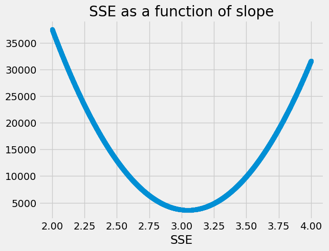
For example, imagine we have the following set of SSE values:

n_slopes = 10000
some_slopes = np.linspace(2, 4, n_slopes)
SSEs = np.zeros(n_slopes)
for i in np.arange(n_slopes):
    SSEs[i] = calc_sse(some_slopes[i])

plt.scatter(some_slopes, SSEs)
plt.xlabel('Slope')
plt.xlabel('SSE')
plt.title('SSE as a function of slope');

We can calculate the matching MSE values by dividing by n (the number of hgb or pcv values).

n = len(hgb)
MSEs = SSEs / n  # Corresponding Mean Square Error

When we plot the MSE values as a function of (y-axis) the SSE values (x axis), we see that there is a straight line relationship, as we would expect, with a slope of 1 / n.

plt.scatter(SSEs, MSEs)
plt.xlabel('SSE values')
plt.ylabel('Corresponding MSE values')
plt.title('MSE as a function of SSE');

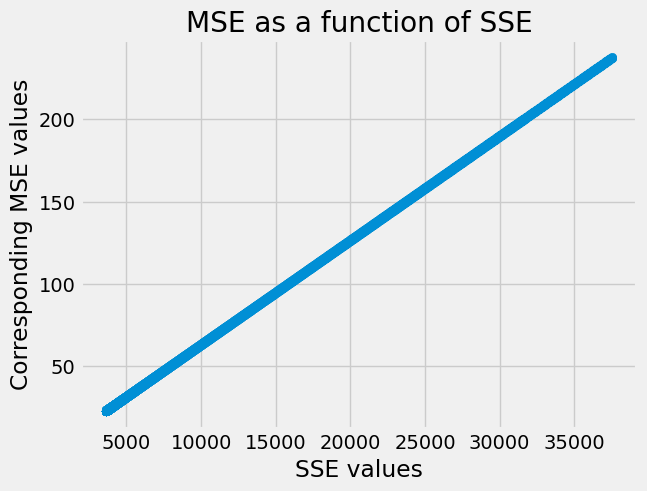
This straight line relationship is one example of a strictly increasing monotonic relationship.

Consider any two SSE values, call these S1 and S2. There are corresponding MSE values M1 and M2 (in fact given by S1 / n and S2 / n). The relationship between SSE and MSE is strictly increasing monotonic because, for any values S1 and S2:

• when S1 > S2 then it is also true thatM1 > M2

• when S1 < S2 then M1 < M2.

• when S1 == S2, M1 == M2.

You can see that relationship in the plot above, because MSE always goes up, as SSE goes up.

The same is true of the RMSE values as a function of the SSE values:

RMSEs = np.sqrt(MSEs)  # Corresponding Root Mean Square Error
plt.scatter(SSEs, RMSEs)
plt.xlabel('SSE values')
plt.ylabel('Corresponding RMSE values')
plt.title('RMSE as a function of SSE');

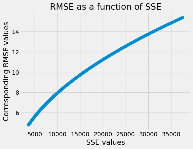
Notice, again, that the RMSE always goes up as SSE goes up.

Now consider minimize. It is looking at the parameters to minimize the value for — say - SSE. But, you can probably see from the argument above, that if we found the parameters to minimize SSE, those must also be the parameters to minimize MSE, and to minimize RMSE, because once we have found the smallest SSE, that must also be the smallest MSE or RMSE.

Therefore, we can minimize on the RMSE, and we are guaranteed to get the same parameters, within calculation precision, as we would if we had minimized on the SSE or the MSE.

In the rest of these textbook pages, we will nearly always use RMSE, because it’s a common metric, and one that is relatively easy to interpret as a typical error for single point.