Finding lines

In The Mean and Slopes, we were looking for the best slope to predict one vector of values from another vector of values.

Specifically, we wanted our slope to predict the Packed Cell Volume (PCV) values from the Hemoglobin (HGB) values.

By analogy with The Mean as Predictor, we decided to choose our line to minimize the average prediction errors, and the sum of squared prediction errors.

We found a solution, by trying many slopes, and choosing the slope giving use the smallest error.

For our question, we were happy to assume that the line passed through 0, 0 — meaning, that when the Hemoglobin is 0, the Packed Cell Volume value is 0. Put another way, we assumed that our line had an intercept value of 0. The intercept is the y value at which the line crosses the y axis, or, put another way, the y value when the x value is 0.

What if we are in a situation where we want to find a line that had a (not zero) intercept, as well as a slope?

import numpy as np
import pandas as pd
pd.set_option('mode.copy_on_write', True)
import matplotlib.pyplot as plt
# Make plots look a little bit more fancy
plt.style.use('fivethirtyeight')
# Print to 4 decimal places, show tiny values as 0
np.set_printoptions(precision=4, suppress=True)

We return to the students ratings dataset dataset.

This is a dataset, in Excel form, where each row is the average of students’ ratings from <RateMyProfessors.com> across a single subject. Thus, the first row refers to the average of all professors teaching English, the second row refers to all professors teaching Mathematics, and so on.

Download the data file via this link rate_my_course.csv.

Next we load the data.

# Read the data file
ratings = pd.read_csv('rate_my_course.csv')
ratings.head()

	Discipline	Number of Professors	Clarity	Helpfulness	Overall Quality	Easiness
0	English	23343	3.756147	3.821866	3.791364	3.162754
1	Mathematics	22394	3.487379	3.641526	3.566867	3.063322
2	Biology	11774	3.608331	3.701530	3.657641	2.710459
3	Psychology	11179	3.909520	3.887536	3.900949	3.316210
4	History	11145	3.788818	3.753642	3.773746	3.053803

We are interested in the relationship of the “Overall Quality” measure to the “Easiness” measure.

# Get the columns as arrays for simplicity and speed.
easiness = np.array(ratings['Easiness'])
quality = np.array(ratings['Overall Quality'])

Do students rate easier courses as being of better quality?

plt.plot(easiness, quality, 'o')
plt.xlabel('Easiness')
plt.ylabel('Overall Quality')

Text(0, 0.5, 'Overall Quality')

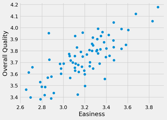
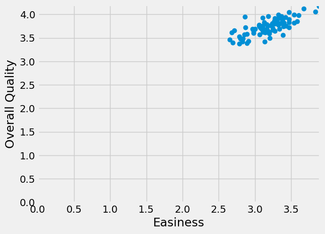
There might be a straight-line relationship here, but it doesn’t look as if it would go through 0, 0:

# The same plot as above, but showing the x, y origin at 0, 0
plt.plot(easiness, quality, 'o')
plt.xlabel('Easiness')
plt.ylabel('Overall Quality')
# Make sure 0, 0 is on the plot.
plt.axis([0, 3.9, 0, 4.2])

(0.0, 3.9, 0.0, 4.2)

In The Mean and Slopes, we assumed that the intercept was zero, so we only had to try different slopes to get our best line.

Here we have a different problem, because we want to find a line that has an intercept that is not zero, so we need to find the best slope and the best intercept at the same time. How do we search for a slope as well as an intercept?

But wait - why do we have to search for the slope and the intercept at the same time? Can’t we just find the best slope, and then the best intercept?

In fact we can’t do that, because the best slope will change for every intercept.

To see why that is, we need to try a few different lines. To do that, we need to remind ourselves about defining lines, and then testing them.

Remember, we can describe a line with an intercept and a slope. Call the intercept \(c\) and a slope \(s\). A line predicts the \(y\) values from the \(x\) values, using the slope \(s\) and the intercept \(c\):

\[ y = c + x * s \]

Let’s start with a guess for the line, just from eyeballing the plot. We guess that:

• The intercept is around 2.25

• The slope is around 0.47

The predicted \(y\) values from this line are (from the formula above):

predicted = 2.25 + easiness * 0.47

where easiness contains our actual \(x\) values.

The prediction error at each point come from the actual \(y\) values minus the predicted \(y\) values.

errors = quality - predicted

where quality contains our actual \(y\) values.

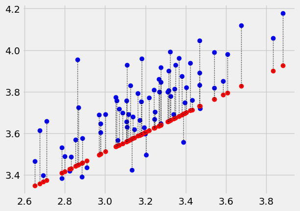
We can look at the predictions for this line (in red), and the actual values (in blue) and then the errors (the lengths of the dotted lines joining the red predictions and the corresponding blue actual values).

# Don't worry about this code.
# It plots the line, and the errors.
x_values = easiness  # The thing we're predicting from, on the x axis
y_values = quality  # The thing we're predicting, on the y axis.
plt.plot(x_values, y_values, 'o')
plt.plot(x_values, predicted, 'o', color='red')
# Draw a line between predicted and actual
for i in np.arange(len(x_values)):
    x = x_values[i]
    y_0 = predicted[i]
    y_1 = y_values[i]
    plt.plot([x, x], [y_0, y_1], ':', color='black', linewidth=1)

The Root Mean Squared Error (RMSE) is:

# Root mean squared error given c and s
rmse_c_s = np.sqrt(np.mean(errors ** 2))
rmse_c_s

0.12027697029219235

Actually, those bits of code are so useful, let’s make them into a function:

def plot_with_errors(x_values, y_values, c, s):
    """ Plot a line through data with errors

    Parameters
    ----------
    x_values : array
        Values we are predicting from, for the x-axis of the plot.
    y_values : array
        Values we are predicting, for the y-axis of the plot.
    c : number
        Intercept for predicting line.
    s : number
        Slope for predicting line.

    Returns
    -------
    rmse : number
        The square root of the mean squared error, for the given `x_values`,
        `y_values` and line.
    """
    # Predict the y values from the line.
    predicted = c + s * x_values
    # Errors are the real values minus the predicted values.
    errors = y_values - predicted
    # Plot real values in blue, predicted values in red.
    plt.plot(x_values, y_values, 'o', color='blue')
    plt.plot(x_values, predicted, 'o', color='red')
    # Draw a line between predicted and actual
    for i in np.arange(len(x_values)):
        x = x_values[i]
        y_0 = predicted[i]
        y_1 = y_values[i]
        plt.plot([x, x], [y_0, y_1], ':', color='black', linewidth=1)
    return np.sqrt(np.mean(errors ** 2))

Notice the string at the top of the function, giving details about what the function does, its arguments, and the values it returns. This is called the docstring. It can remind you and other people what the function does, and how to use it. Try making a new cell and type plot_with_errors?. You’ll see this string is the help that Python will fetch for this function.

Now the same thing with the function:

plot_with_errors(easiness, quality, 2.25, 0.47)

0.12027697029219235

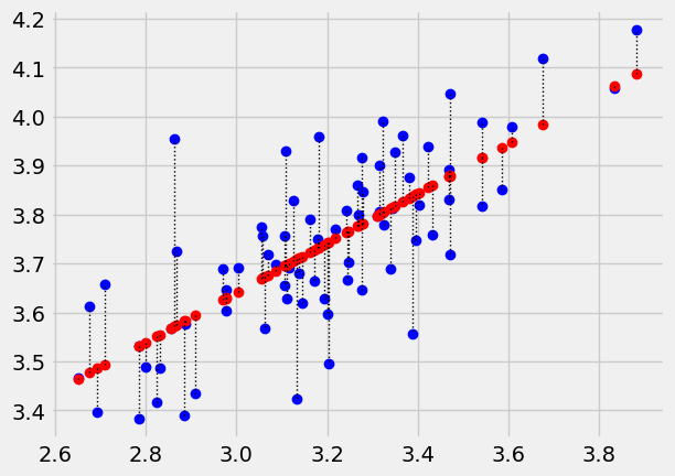
If we try a different intercept, we’ll get a different line, and a different error. Let’s try an intercept of 2.1:

plot_with_errors(easiness, quality, 2.1, 0.47)

0.18316435491606842

Or, we could go back to the same intercept, but try a different slope, and we’d get a different error. Let’s try a slope of 0.5:

plot_with_errors(easiness, quality, 2.25, 0.5)

0.16024697296024795

Now we use the long slow method to find the best slope for our initial intercept of 2.25. You may recognize the following from the mean and slopes notebook.

First we make a function, a bit like the function above, that gives us the error for any given intercept (c) and slope (s) like this:

def calc_rmse_for_c_s(c, s):
    predicted_quality = c + easiness * s
    errors = quality - predicted_quality
    return np.sqrt(np.mean(errors ** 2))

We have already calculated the error for the original guess at slope and intercept, but let’s do it again for practice:

# RMSE for our initial guessed line.
predicted = 2.25 + easiness * 0.47
error = quality - predicted
np.sqrt(np.mean(error ** 2))

0.12027697029219235

Check that our function gives the same value for the same intercept and slope:

calc_rmse_for_c_s(2.25, 0.47)

0.12027697029219235

OK, now we use this function to try lots of different slopes, for this intercept, and see which slope gives us the lowest error. See the means, slopes notebook for the first time we did this.

some_slopes = np.arange(-2, 2, 0.001)
slope_df = pd.DataFrame()
slope_df['slope_to_try'] = some_slopes
slope_df

	slope_to_try
0	-2.000
1	-1.999
2	-1.998
3	-1.997
4	-1.996
...	...
3995	1.995
3996	1.996
3997	1.997
3998	1.998
3999	1.999

4000 rows × 1 columns

As for the mean and slopes notebook, we make an array to hold the RMSE results for each slope.

# Number of slopes.
n_slopes = len(some_slopes)
# Array to store the RMSE for each slope.
rmses = np.zeros(n_slopes)

Then (as before) we calculate and store the RMSE value for each slope, with this given intercept.

# Try all these slopes for an intercept of 2.25
for i in np.arange(n_slopes):  # For each candidate slope.
    # Get the corresponding slope.
    this_slope = some_slopes[i]
    # Calculate the error measure for this slope and intercept 2.25.
    this_error = calc_rmse_for_c_s(2.25, this_slope)
    # Put the error into the results array at the corresponding position.
    rmses[i] = this_error

# Put all the RMSE scores into the DataFrame as a column for display.
slope_df['RMSE'] = rmses
slope_df

	slope_to_try	RMSE
0	-2.000	7.885813
1	-1.999	7.882617
2	-1.998	7.879421
3	-1.997	7.876225
4	-1.996	7.873028
...	...	...
3995	1.995	4.886684
3996	1.996	4.889880
3997	1.997	4.893075
3998	1.998	4.896271
3999	1.999	4.899466

4000 rows × 2 columns

We plot the errors we got for each slope, and find the slope giving the smallest error:

plt.plot(slope_df['slope_to_try'], slope_df['RMSE'])
plt.xlabel('Candidate slopes')
plt.ylabel('Root mean squared error')

Text(0, 0.5, 'Root mean squared error')

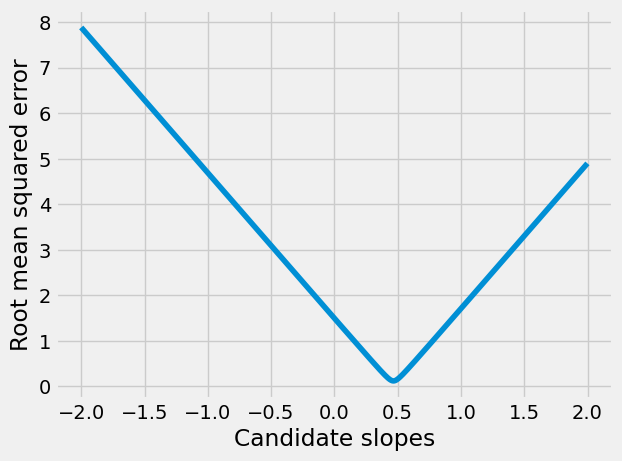
Find the row corresponding to the smallest RMSE:

# Row label corresponding to minimum value.
row_with_min = slope_df['RMSE'].idxmin()
slope_df.loc[row_with_min]

slope_to_try    0.46700
RMSE            0.11982
Name: 2467, dtype: float64

# Slope giving smallest RMSE for intercept 2.25
slope_df.loc[row_with_min, 'RMSE']

0.119820093530566

OK — that’s the best slope for an intercept of 2.25. How about our other suggestion, of an intercept of 2.1? Let’s try that:

# Try all candidate slopes for an intercept of 2.1.
# We will reuse "rmses" and "slope_df" for simplicity.
for i in np.arange(n_slopes):  # For each candidate slope.
    # Get the corresponding slope.
    this_slope = some_slopes[i]
    # Calculate the error measure for this slope and intercept 2.21.
    this_error = calc_rmse_for_c_s(2.1, this_slope)
    # Put the error into the results array at the corresponding position.
    rmses[i] = this_error

# Put all the RMSE scores into the DataFrame as a column for display.
slope_df['RMSE'] = rmses
slope_df

	slope_to_try	RMSE
0	-2.000	8.035281
1	-1.999	8.032085
2	-1.998	8.028889
3	-1.997	8.025693
4	-1.996	8.022497
...	...	...
3995	1.995	4.737225
3996	1.996	4.740420
3997	1.997	4.743616
3998	1.998	4.746811
3999	1.999	4.750007

4000 rows × 2 columns

# Recalculate row holding minimum RMSE
row_with_min_for_2p1 = slope_df['RMSE'].idxmin()
slope_df.loc[row_with_min_for_2p1]

slope_to_try    0.513000
RMSE            0.119317
Name: 2513, dtype: float64

Oh dear - the best slope has changed. And, in general, for any intercept, you may able to see that the best slope will be different, as the slope tries to adjust for the stuff that the intercept does not explain.

This means we can’t just find the intercept, and find the best slope for that intercept, at least not in our case - we have to find the best pair of intercept and slope. This is the pair, of all possible pairs, that gives the lowest error.

Our task then, is to find the pair of values — c and s — such that we get the smallest possible value for the root mean squared errors above.

One way of doing this, is to try every possible plausible pair of intercept and slope, calculate the error for this pair, and then find the pair that gave the lowest error.

We are now searching over many pairs of slopes and intercepts.

Here are some candidate intercepts to try:

# Some intercepts to try
some_inters = np.arange(1, 3.2, 0.01)
inter_df = pd.DataFrame()
inter_df['intercept_to_try'] = some_inters
inter_df

	intercept_to_try
0	1.00
1	1.01
2	1.02
3	1.03
4	1.04
...	...
215	3.15
216	3.16
217	3.17
218	3.18
219	3.19

220 rows × 1 columns

We would like to calculate RMSE values for all combinations of slopes and intercepts. That is, we want to get RMSE values for all slopes, for the first intercept value (1), and RMSE values for all slopes, and the second intercept value (1.01), and so on.

We have:

print('Number of slopes to try:', n_slopes)
n_inters = len(some_inters)
print('Number of intercepts to try:', n_inters)
n_pairs = n_slopes * n_inters
print('Number of pairs to try:', n_pairs)

Number of slopes to try: 4000
Number of intercepts to try: 220
Number of pairs to try: 880000

To do this, we could make a new DataFrame with one row per intercept, slope pair. The intercept column inter_to_try will have the intercept values, and the second slope_to_try will have the slope values.

Let’s repeat each intercept value n_slopes times, using np.repeat. As you remember, np.repeat repeats each element in the array by a given number of times:

# Repeat each element in the array 3 times.
np.repeat([1, 2, 3], 3)

array([1, 1, 1, 2, 2, 2, 3, 3, 3])

To make the column of intercepts we repeat each element of the intercepts array n_slopes times:

pair_df = pd.DataFrame()
repeated_inters = np.repeat(some_inters, n_slopes)
# Show in DataFrame
pair_df['inter_to_try'] = repeated_inters
pair_df

	inter_to_try
0	1.00
1	1.00
2	1.00
3	1.00
4	1.00
...	...
879995	3.19
879996	3.19
879997	3.19
879998	3.19
879999	3.19

880000 rows × 1 columns

To make the slope_to_try column, we need to repeat the whole some_slopes array n_inters times. Notice that np.repeat repeats each element a given number of times. To repeat the whole array, we can use np.tile, like this:

# Repeat the whole array 3 times.
np.tile([1, 2, 3], 3)

array([1, 2, 3, 1, 2, 3, 1, 2, 3])

To repeat the whole some_slopes array n_inters times:

tiled_slopes = np.tile(some_slopes, n_inters)
# Show in DataFrame
pair_df['slope_to_try'] = tiled_slopes
pair_df

	inter_to_try	slope_to_try
0	1.00	-2.000
1	1.00	-1.999
2	1.00	-1.998
3	1.00	-1.997
4	1.00	-1.996
...	...	...
879995	3.19	1.995
879996	3.19	1.996
879997	3.19	1.997
879998	3.19	1.998
879999	3.19	1.999

880000 rows × 2 columns

The rows of this DataFrame (and the arrays that went into them) define all the possible intercept, slope pairs.

We next make another array to contains the RMSE values for each pair.

# An array to store the RMSE values for each intercept, slope pair.
pair_rmses = np.zeros(n_pairs)

We can use these arrays to go through each slope, intercept pair in turn, calculate the RMSE, and store it for later use.

# Go through each pair to calculate the corresponding RMSE.
# (Or, equivalently, go through the values for each row in the `pair_df`
# DataFrame).
for i in np.arange(n_pairs):
    # Get the intercept for this pair (intercept at this position).
    this_intercept = repeated_inters[i]
    # Get the slope for this pair (slope at this position).
    this_slope = tiled_slopes[i]
    # Calculate the error measure.
    this_error = calc_rmse_for_c_s(this_intercept, this_slope)
    # Put the error into the RMSE results array at this position.
    pair_rmses[i] = this_error

# Add the RMSE column to the original DataFrame for display.
pair_df['RMSE'] = pair_rmses
pair_df

	inter_to_try	slope_to_try	RMSE
0	1.00	-2.000	9.131916
1	1.00	-1.999	9.128720
2	1.00	-1.998	9.125524
3	1.00	-1.997	9.122328
4	1.00	-1.996	9.119132
...	...	...	...
879995	3.19	1.995	5.823930
879996	3.19	1.996	5.827125
879997	3.19	1.997	5.830321
879998	3.19	1.998	5.833516
879999	3.19	1.999	5.836712

880000 rows × 3 columns

For each of the n_inters possible intercepts, we have tried all n_slopes possible slopes, and we have found the RMSE for each intercept, slope pair. We can now find the pair that gives the lowest RMSE.

# The lowest error that we found for any slope, intercept pair
min_row_label = pair_df['RMSE'].idxmin()
best_row = pair_df.loc[min_row_label]
best_row

inter_to_try    2.120000
slope_to_try    0.507000
RMSE            0.119304
Name: 450507, dtype: float64

Notice that the error (RMSE) for this pair is lower than the error we found for our guessed c and s:

calc_rmse_for_c_s(2.25, 0.47)

0.12027697029219235

# The intercept corresponding to the lowest error
best_intercept = best_row['inter_to_try']
best_slope = best_row['slope_to_try']
print('Best intercept, slope pair:', best_intercept, best_slope)

Best intercept, slope pair: 2.120000000000001 0.5069999999997239

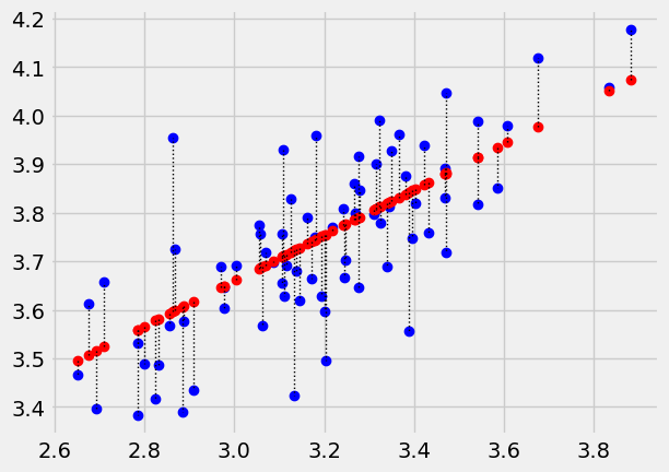
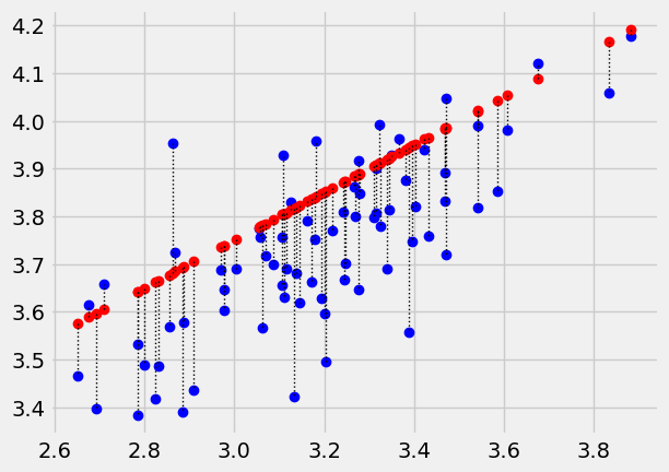
Plot the data, predictions and errors for the line that minimizes the sum of squared error:

plot_with_errors(easiness, quality, best_intercept, best_slope)

0.11930386031906048

Now you know about optimization, you will not be surprised to discover that Scipy minimize can also do the search for the intercept and slope pair for us. We send minimize the function we are trying to minimize, and a starting guess for the intercept and slope.

minimize is a little fussy about the functions it will use. It insists that all the parameters need to be passed in as a single argument. In our case, we need to pass both parameters (the intercept and slope) as one value, containing two elements, like this:

def calc_rmse_for_minimize(c_s):
    # c_s has two elements, the intercept c and the slope s.
    c = c_s[0]
    s = c_s[1]
    predicted_quality = c + easiness * s
    errors = quality - predicted_quality
    return np.sqrt(np.mean(errors ** 2))

This is the form of the function that minimize can use. See using minimize for more detail.

We first confirm this gives us the same answer we got before from our function with two arguments:

# The original function
calc_rmse_for_c_s(2.25, 0.47)

0.12027697029219235

# The function in the form that minimize wants
# The two parameters go into a list, that we can pass as a single argument.
calc_rmse_for_minimize([2.25, 0.47])

0.12027697029219235

As usual with minimize we need to give a starting guess for the intercept and slope. We will start with our initial guess of [2.25, 0.47], but any reasonable guess will do.

from scipy.optimize import minimize
minimize(calc_rmse_for_minimize, [2.25, 0.47])

  message: Optimization terminated successfully.
  success: True
   status: 0
      fun: 0.11930057876222537
        x: [ 2.115e+00  5.089e-01]
      nit: 4
      jac: [-2.442e-06  1.345e-06]
 hess_inv: [[ 1.773e+01 -5.527e+00]
            [-5.527e+00  1.735e+00]]
     nfev: 24
     njev: 8

Notice that minimize doesn’t get exactly the same result as we found with the long slow way above. This is because the long slow way only tested intercepts that were step-sizes of 0.01 apart (and slopes that were 0.001 apart). minimize can use much smaller step-sizes, and so finds a more accurate answer.

We won’t spend any time justifying this, but this is also the answer we get from traditional fitting of the least-squares line, as implemented, for example, in the Scipy linregress function:

from scipy.stats import linregress
linregress(easiness, quality)

LinregressResult(slope=0.5088641203940006, intercept=2.114798571643314, rvalue=0.7459725836595872, pvalue=1.5998303978986516e-14, stderr=0.053171209477256925, intercept_stderr=0.1699631063847937)

Notice the values for slope and intercept in the output above.