Selecting columns from DataFrames

# Load the Pandas data science library, call it 'pd'
import pandas as pd
# Turn on a setting to use Pandas more safely.
# We will discuss this setting later.
pd.set_option('mode.copy_on_write', True)

# Load the library for plotting, name it 'plt'
import matplotlib.pyplot as plt
# Make plots look a little more fancy
plt.style.use('fivethirtyeight')

Let us return to the DataFrame we had at the end of the previous notebook The data frame index.

# Original data frame before dropping missing values.
gender_data = pd.read_csv('gender_stats_min.csv')
gender_data_no_na = gender_data.dropna()
labeled_gdata = gender_data_no_na.set_index('country_code')
# Show the result
labeled_gdata

	country_name	gdp_us_billion	mat_mort_ratio	population
country_code
AFG	Afghanistan	19.961015	444.00	32.715838
AGO	Angola	111.936542	501.25	26.937545
ALB	Albania	12.327586	29.25	2.888280
ARE	United Arab Emirates	375.027082	6.00	9.080299
ARG	Argentina	550.980968	53.75	42.976675
...	...	...	...	...
WSM	Samoa	0.799887	54.75	0.192225
YEM	Yemen, Rep.	36.819337	399.75	26.246608
ZAF	South Africa	345.209888	143.75	54.177209
ZMB	Zambia	24.280990	233.75	15.633220
ZWE	Zimbabwe	15.495514	398.00	15.420964

179 rows × 4 columns

Selecting columns

You have seen array indexing (in Selecting with arrays. You remember that array indexing uses square brackets. Indexing is the technical term for getting data from a value using square brackets. Data frames also allow indexing. For example, we often want to get all the data for a single column of the data frame. To do this, we use the same square bracket notation as we use for array indexing, with the name of the column inside the square brackets.

gdp = labeled_gdata['gdp_us_billion']

Call this column label indexing.

We all also call this direct indexing with column labels or DICL.

By direct indexing we mean indexing a DataFrame using square brackets after the DataFrame value — the kind of indexing you will be familiar with from arrays. Later we will come across another form of indexing, called indirect indexing, but that is for another time.

What type of value came back from this direct indexing with column labels?

type(gdp)

pandas.core.series.Series

Pandas sent back a Series value from our selection of the column. The Series is a Pandas’ way of representing a column of data. Here is the default display for the gdp Series:

gdp

country_code
AFG     19.961015
AGO    111.936542
ALB     12.327586
ARE    375.027082
ARG    550.980968
          ...    
WSM      0.799887
YEM     36.819337
ZAF    345.209888
ZMB     24.280990
ZWE     15.495514
Name: gdp_us_billion, Length: 179, dtype: float64

The display shows the values from the column, that you saw previously in the DataFrame gdp_us_billion column. You see the values printed on the right. Notice too that the Series has kept the row labels from the DataFrame, so each value now has it’s corresponding row label. The index values are on the left.

Notice that, if your string specifying the column name does not match a column name exactly, you will get a long error. This gives you some practice in reading long error messages - skip to the end first, you will often see the most helpful information there.

# The correct column name is in lower case.
labeled_gdata['GDP_US_BILLION']

---------------------------------------------------------------------------
KeyError                                  Traceback (most recent call last)
File /opt/hostedtoolcache/Python/3.11.8/x64/lib/python3.11/site-packages/pandas/core/indexes/base.py:3805, in Index.get_loc(self, key)
   3804 try:
-> 3805     return self._engine.get_loc(casted_key)
   3806 except KeyError as err:

File index.pyx:167, in pandas._libs.index.IndexEngine.get_loc()

File index.pyx:196, in pandas._libs.index.IndexEngine.get_loc()

File pandas/_libs/hashtable_class_helper.pxi:7081, in pandas._libs.hashtable.PyObjectHashTable.get_item()

File pandas/_libs/hashtable_class_helper.pxi:7089, in pandas._libs.hashtable.PyObjectHashTable.get_item()

KeyError: 'GDP_US_BILLION'

The above exception was the direct cause of the following exception:

KeyError                                  Traceback (most recent call last)
Cell In[6], line 2
      1 # The correct column name is in lower case.
----> 2 labeled_gdata['GDP_US_BILLION']

File /opt/hostedtoolcache/Python/3.11.8/x64/lib/python3.11/site-packages/pandas/core/frame.py:4090, in DataFrame.__getitem__(self, key)
   4088 if self.columns.nlevels > 1:
   4089     return self._getitem_multilevel(key)
-> 4090 indexer = self.columns.get_loc(key)
   4091 if is_integer(indexer):
   4092     indexer = [indexer]

File /opt/hostedtoolcache/Python/3.11.8/x64/lib/python3.11/site-packages/pandas/core/indexes/base.py:3812, in Index.get_loc(self, key)
   3807     if isinstance(casted_key, slice) or (
   3808         isinstance(casted_key, abc.Iterable)
   3809         and any(isinstance(x, slice) for x in casted_key)
   3810     ):
   3811         raise InvalidIndexError(key)
-> 3812     raise KeyError(key) from err
   3813 except TypeError:
   3814     # If we have a listlike key, _check_indexing_error will raise
   3815     #  InvalidIndexError. Otherwise we fall through and re-raise
   3816     #  the TypeError.
   3817     self._check_indexing_error(key)

KeyError: 'GDP_US_BILLION'

GDP and Maternal Mortality Rate

There are two ways of getting plots from data in data frames. Here we use the most basic method, that you have already seen. Soon, we will get onto a more elegant plotting method.

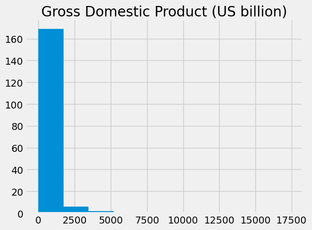
The gdp variable is a sequence of values, so we can do a histogram on these values, as we have done histograms on arrays.

plt.hist(gdp)
plt.title('Gross Domestic Product (US billion)');

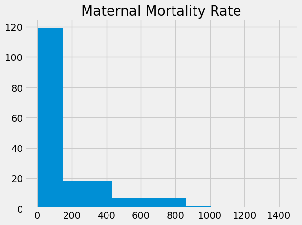
Now we have had a look at the GDP values, we will look at the values for the Maternal Mortality Rate (MMR). The MMR is the number of women who die in childbirth for every 100,000 births. These are the numbers in the mat_mort_ratio column.

mmr = labeled_gdata['mat_mort_ratio']
mmr

country_code
AFG    444.00
AGO    501.25
ALB     29.25
ARE      6.00
ARG     53.75
        ...  
WSM     54.75
YEM    399.75
ZAF    143.75
ZMB    233.75
ZWE    398.00
Name: mat_mort_ratio, Length: 179, dtype: float64

Notice the row labels on the left, and the values from the mat_mort_ratio column on the right.

plt.hist(mmr)
plt.title('Maternal Mortality Rate');

Selecting more than one column

Let us say that we would like to avoid distraction by restricting our data frame to the columns we are interested in.

There are our columns labels:

col_labels = list(labeled_gdata)
col_labels

['country_name', 'gdp_us_billion', 'mat_mort_ratio', 'population']

Let us say that, for now, we only want the first three columns. We can do that with direct indexing with column labels (DICL) too. To do that, we put a list of strings between the square brackets, instead of the string with the column name.

Here are the column labels we want:

# Select all labels but the last.
col_labels_we_want = col_labels[:-1]
col_labels_we_want

['country_name', 'gdp_us_billion', 'mat_mort_ratio']

We can select only these columns using direct indexing:

# Direct indexing with a list of column labels
thinner_gdata = labeled_gdata[col_labels_we_want]
thinner_gdata

	country_name	gdp_us_billion	mat_mort_ratio
country_code
AFG	Afghanistan	19.961015	444.00
AGO	Angola	111.936542	501.25
ALB	Albania	12.327586	29.25
ARE	United Arab Emirates	375.027082	6.00
ARG	Argentina	550.980968	53.75
...	...	...	...
WSM	Samoa	0.799887	54.75
YEM	Yemen, Rep.	36.819337	399.75
ZAF	South Africa	345.209888	143.75
ZMB	Zambia	24.280990	233.75
ZWE	Zimbabwe	15.495514	398.00

179 rows × 3 columns

Dropping columns

We have just used DICL to select the columns we want. In the case above, we selected three out of the four column labels, and our DICL operation had the effect of dropping the last column.

Another way of dropping a column is to use the DataFrame .drop method.

In fact the .drop method allows us to drop columns and rows. To tell .drop we want to drop columns rather than rows, we use the column= keyword argument to .drop, like this:

# Drop the population column.
thinner_again = labeled_gdata.drop(columns=['population'])
thinner_again

	country_name	gdp_us_billion	mat_mort_ratio
country_code
AFG	Afghanistan	19.961015	444.00
AGO	Angola	111.936542	501.25
ALB	Albania	12.327586	29.25
ARE	United Arab Emirates	375.027082	6.00
ARG	Argentina	550.980968	53.75
...	...	...	...
WSM	Samoa	0.799887	54.75
YEM	Yemen, Rep.	36.819337	399.75
ZAF	South Africa	345.209888	143.75
ZMB	Zambia	24.280990	233.75
ZWE	Zimbabwe	15.495514	398.00

179 rows × 3 columns

Back to GDP and MMR

We are interested in the relationship of gpp and mmr. Maybe richer countries have better health care, and fewer maternal deaths.

Here is a plot, using the standard Matplotlib scatter function.

plt.scatter(gdp, mmr);
plt.title('Maternal Mortality Rate as a function of GDP');

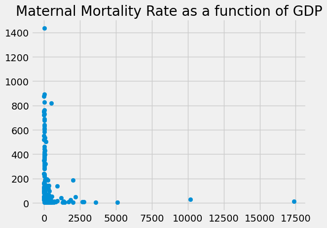
The scatterplot is not convincing in showing a relationship between GDP and the MMR. That is puzzling, given the assumption that higher GDP tends to be associated with better healthcare.

We need to explore some more. For example, could it be that, beyond a certain level of GDP, healthcare is good enough to prevent most maternal deaths? In that case, we might still expect a relationship between GDP and MMR in lower-income countries, but a much weaker relationship for lower-income countries.

To go further, we will see what we can do by sorting the DataFrame, and looking at the first and last rows.