Confident treatment#
Show code cell content
# Run this cell; do not change it.
import numpy as np
# Make random number generator.
rng = np.random.default_rng()
import pandas as pd
pd.set_option('mode.copy_on_write', True)
# Make printing of numbers a bit neater.
np.set_printoptions(precision=4, suppress=True)
import matplotlib.pyplot as plt
# Make the plots look more fancy.
plt.style.use('fivethirtyeight')
How confident can we be that a treatment works?
At the time I wrote this, you can find the following on the Wikipedia page for Burkitt’s Lymphoma.
The overall cure rate for Burkitt’s lymphoma in developed countries is about 90%, but worse in low-income countries. Burkitt’s lymphoma is uncommon in adults, where it has a worse prognosis (Molyneux et al 2012).
In 2006, treatment with dose-adjusted EPOCH with Rituximab showed promising initial results in a small series of patients (n=17), with a 100% response rate, and 100% overall survival and progression-free survival at 28 months (median follow-up) (Dunleavy et al 2006).
Molyneux et al (2012). Burkitt’s Lymphoma. The Lancet, 379(9822), 1234-1244.
Dunleavy et al (2006). Novel Treatment of Burkitt Lymphoma with Dose-Adjusted EPOCH-Rituximab: Preliminary Results Showing Excellent Outcome. Blood, 108(11), 2736–2736.
Now I have the following questions. Given the trial data above:
How likely is it that the Rituximab treatment is always effective (100%)?
How likely is it that Rituximab is less effective than standard treatment (less than 90% effective)?
How are we going to answer these questions?
First we go back to the calculations we do know. We have previously calculated (by simulation) the chance that we will see this 17/17 result, given that the treatment is in fact 90% effective.
Let’s do that again:
#- Simulate 100000 trials of 17 patients
n_iters = 100000
counts = np.zeros(n_iters)
for i in np.arange(n_iters):
    cured = rng.choice([0, 1], p=[0.1, 0.9], size=17)
    counts[i] = np.count_nonzero(cured)
p_observed = np.count_nonzero(counts == 17) / n_iters
p_observed
0.16668
Now we let you into a secret; you can get an exact value for this probability by using something called the binomial distribution. We will not explain why that is the case, because it is not important for our purposes, but we can get the exact result corresponding to our estimate from simulation with:
from scipy.stats import binom

n_obs = 17   # The number of observations (here, patients).
p_success = 0.9  # The probability of success on every trial (patient).
n_successes = 17   # The number of successes we want a probability for.

# Exact calculation for probability we got by simulation.
exact_for_90 = binom.pmf(n_successes, n_obs, p_success)
exact_for_90
0.16677181699666577
Let’s confirm the simulation above really does give about the same value as
the binom trick, by trying a simulation in a world where there is a 95% cure rate.
counts = np.zeros(n_iters)
for i in np.arange(n_iters):
    cured = rng.choice([0, 1], p=[0.05, 0.95], size=17)
    counts[i] = np.count_nonzero(cured)
p_observed_95 = np.count_nonzero(counts == 17) / n_iters
p_observed_95
0.4188
And with binom:
# Exact calculation for probability we got by simulation.
exact_for_95 = binom.pmf(n_successes, n_obs, 0.95)
exact_for_95
0.4181203352191771
In fact we can use binom to calculate both probabilities at the same time by
passing an array to the probability argument:
# Exact calculation for two worlds
exact_for_both = binom.pmf(n_successes, n_obs, np.array([0.9, 0.95]))
Some notation#
Call the 17/17 result \(C_{17}\) (for “17 cured”). Call the world where the treatment is 90% effective \(T_{90}\).
In our first simulation we found the probability of seeing \(C_{17}\) in a \(T_{90}\) world:
p_c17_given_t90 = exact_for_90
We’ve also got the equivalent value for a \(T_{95}\) world:
p_c17_given_t95 = exact_for_95
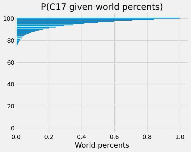
Let’s calculate the probability value for all positive integer percentages:
world_percents = np.arange(1, 101)
world_probs = world_percents / 100
p_c17_given_worlds = binom.pmf(n_successes, n_obs, world_probs)
plt.barh(world_percents, p_c17_given_worlds)
plt.xlabel('World percents')
plt.title('P(C17 given world percents)');
Now we want to do our Bayes calculation, but we are missing something. We do not have the prior probability of each world percent for this treatment.
Maybe the true world percent is the standard percent — 90% — and the treatment is no more effective than average. Or maybe the true world percent is 100%. How do we know where to start with our probabilities for each world — \(P(T_{90})\), \(P(T_{100})\) and so on?
Let’s start somewhere. Let’s say we have no idea what the true world probabilities are, so we will make all the initial probabilities the same. We have 100 world percentages we are interested in, so the probability of each world is 1/100. With that assumption, we can do our Bayes calculation.
worlds = pd.DataFrame()
# Same probability for each treatment world.
n_worlds = len(world_percents)
worlds['P(T)'] = np.ones(n_worlds) * 1 /n_worlds
worlds['P(C17 given T)'] = p_c17_given_worlds
worlds['P(T and C17)'] = worlds['P(T)'] * worlds['P(C17 given T)']
worlds['P(T given C17)'] = (worlds['P(T and C17)'] /
                            worlds['P(T and C17)'].sum())
# Use the percent values for the world as the row labels.
worlds.index = world_percents
worlds.tail()
| P(T) | P(C17 given T) | P(T and C17) | P(T given C17) | |
|---|---|---|---|---|
| 96 | 0.01 | 0.499587 | 0.004996 | 0.082308 |
| 97 | 0.01 | 0.595826 | 0.005958 | 0.098164 |
| 98 | 0.01 | 0.709322 | 0.007093 | 0.116862 |
| 99 | 0.01 | 0.842943 | 0.008429 | 0.138877 |
| 100 | 0.01 | 1.000000 | 0.010000 | 0.164752 |
short_worlds = worlds.tail(20)  # Just show the 80% - 100%
short_worlds.plot.barh(subplots=True, legend=False);
plt.subplots_adjust(hspace=0.8)  # Space out the plots.
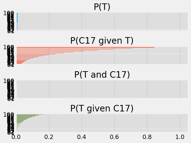
With these assumptions, we can give some answers to our questions.
The probability of this treatment having 100% cure rate is:
worlds.loc[100, 'P(T given C17)']
0.1647523390001275
The probability that the treatment is less than 90% effective is:
worlds.loc[worlds.index < 90, 'P(T given C17)'].sum()
0.12407449105131524
You might well be thinking to yourself — what about a treatment world with
99.5% response rate? We can solve this too, by using finer percent intervals
than we used in world_percents above. Try it!