Bayes theorem#
The reverse probability page has a game, that we analyzed by simulation, and then by reflection.
The game is:
I have two boxes; BOX4 with 4 red balls and 1 green ball, and BOX2 with two red balls and three green balls.
I offer you one of these two boxes, with a 30% chance that I give you BOX4, and 70% chance I give you BOX2.
You draw a ball at random from the box, and you get a red ball.
What is the probability that I gave you BOX4?
We found by simulation, and later by reflection, that the probability is about 0.462.
The logic we discovered was:
We want the proportion of “red” trials that came from BOX4.
Calculate the proportion of trials that are both BOX4 and red, and divide by the overall proportion of red trials.
Here is a Sankey diagram of that calculation:
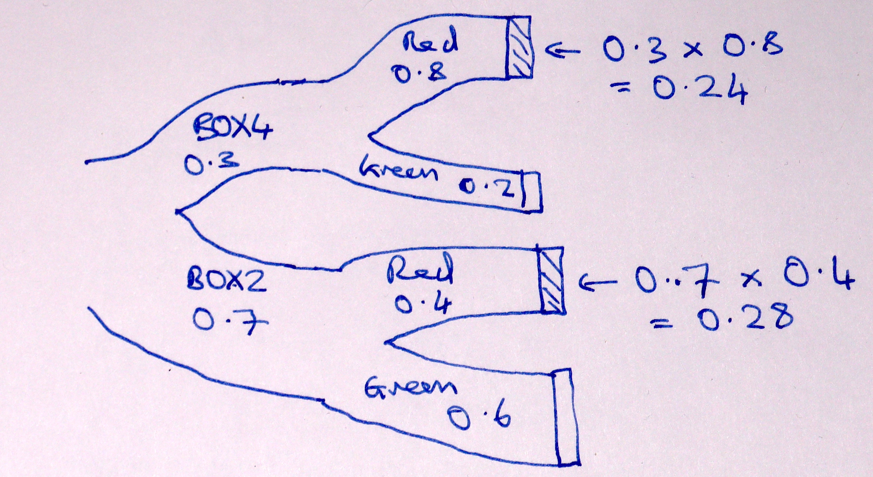
We found the proportion of red trials that are both BOX4 and red is (the proportion of BOX4 trials) multiplied by (the proportion of BOX4 trials that are red.
In our case above, the value we need is the probability of red trials from BOX4 (red AND BOX4) divided by the probability of red from either box. In our case this is 0.24 / (0.24 + 0.28) = 0.4615.
The logic above is a fundamental rule in probability called Bayes theorem.
In this page, we relate the logic above to the usual way of describing Bayes theorem.
First we need some notation.
The probability that I give you BOX4 on any one trial is 0.3.
I could write this out long-hand as “probability of BOX4”, but this will soon become inconvenient, so I will write the “probability of BOX4” in a much more compact form as \(P(B4)\). As you remember \(P(B4)\) is 0.3:
Read this as “the probability of BOX4 is 0.3”.
Similarly:
The probability of getting a red ball, given that I am drawing from BOX4, is 4/5 = 0.8. Again, we could write that out longhand as “probability of red given BOX4, or:
but I want to make this more compact. First I will shorten \(\mathrm{red}\) to \(R\), and then I will write “given” with the bar: \(\mid\).
Read this as “the probability of drawing a red ball given I have BOX4 is 0.8”.
Similarly:
“The probability of red given BOX2 is 0.4”.
We follow the logic above, with this notation. Here is the logic again:
We want the proportion of “red” trials that came from BOX4.
Calculate the proportion of trials that are both BOX4 and red, and divide by the overall proportion of red trials.
We can express the first statement by saying that we are trying to find \(P(B4 \mid R)\) — “the probability of BOX4 given I have drawn a red ball”.
Now we need some more notation. We need the idea of the probability of getting both BOX4 and red. This is the probability for any one trial that we will end up with a red from BOX4, as opposed to a red from BOX2 or a green from either box.
We could write this as and \(P(B4\ \mathrm{and}\ R)\), but in fact, we usually shorten the and to this symbol: \(\cap\):
Read this as the “probability we got BOX4 and then a red”.
We have already found that that we get this probability of BOX4 and red by multiplying the probability of BOX4 (0.3) by the probability of — getting a red ball, given BOX4 (0.8). In our notation, this multiplication is
“The probability of BOX4 and red is the probability of BOX4 multiplied by the probability of — red given BOX4”.
Remember too, from the reverse probability page that we found \(P(R)\) by adding the probabilities of the two different ways we can get a red ball: \(P(R) = P(R \mid B4) + P(R \mid B2)\).
Let’s put all that on the Sankey diagram:

Putting the first and second statements together into one, we get:
This is Bayes theorem, although it is usually written with the multiplication in the other order:
See Bayes theorem on Wikipedia for more detail.