Permutations and pairs

Sometimes the difference we are interested in is a difference between pairs of values.

In the idea of permutation page, we introduced data from an experiment on effect of drinking beer on mosquitoes. These data are a good example of a situation where we want to look at differences between pairs of values.

You may remember that the experiment involved two groups of participants. A group of 24 participants drank beer for the experiment, and another group of 18 subjects drank water. The experimenters took a measure of how attractive each person was to mosquitoes. Specifically they put each person in a tent, from which there was an air tube leading to a closed box of 50 mosquitoes. The experimenters then opened the box and counted how many mosquitoes flew down the tube towards the tent containing the person. This count is the “activated” column in the dataset.

In fact, they did this procedure twice for each volunteer, once before they drank their allocated drink, and once after. The difference between before and after is a measure of the difference to the mosquitoes after the subject had had their drink.

Without further ado, let us load the data.

If you want to run this notebook on your own computer, Download the data from mosquito_beer.csv.

See this page for more details on the dataset, and the data license page.

# Import Numpy library, rename as "np"
import numpy as np
# Make random number generator.
rng = np.random.default_rng()
# Import Pandas library, rename as "pd"
import pandas as pd
# Safe setting for Pandas.
pd.set_option('mode.copy_on_write', True)

# Set up plotting
import matplotlib.pyplot as plt
plt.style.use('fivethirtyeight')

mosquitoes = pd.read_csv('mosquito_beer.csv')
mosquitoes.head()

	volunteer	group	test	nb_released	no_odour	volunt_odour	activated	co2no	co2od	temp	trapside	datetime
0	subj1	beer	before	50	7	9	16	305.0	321.0	36.1	A	2007-08-28 19:00:00
1	subj2	beer	before	50	26	7	33	338.0	720.0	35.3	B	2007-08-28 21:00:00
2	subj3	beer	before	50	5	10	15	348.0	355.0	36.1	B	2007-09-15 19:00:00
3	subj4	beer	before	50	3	7	10	349.0	437.0	35.6	A	2007-09-25 17:00:00
4	subj5	beer	before	50	2	8	10	396.0	475.0	37.0	B	2007-09-25 18:00:00

As you saw above, the experimental procedure left us with two mosquito counts for each volunteer, one count taken before they had had their drink, and another count after.

Here we collect those before and after values for each beer-drinking volunteer. Please ignore the code below, we will cover this kind of data selection and organization later in the course.

# Make new DataFrame with before and after for each volunteer.
# Run this cell for now.  We will cover this code later in the course.
# Just the beer drinkers.
beer = mosquitoes[mosquitoes['group'] == 'beer']
before = beer[beer['test'] == 'before']
after = beer[beer['test'] == 'after']
# Merge before and after rows for matching volunteers.
both = before.merge(after, on=['volunteer', 'group'],
                    suffixes=['_before', '_after'])
# Select the columns we're interested in.
before_after = both[['group', 'activated_before', 'activated_after']]
before_after

	group	activated_before	activated_after
0	beer	16	14
1	beer	33	33
2	beer	15	27
3	beer	10	11
4	beer	10	12
5	beer	30	27
6	beer	15	26
7	beer	17	25
8	beer	23	27
9	beer	8	27
10	beer	31	22
11	beer	15	36
12	beer	26	37
13	beer	5	3
14	beer	18	23
15	beer	12	7
16	beer	22	25
17	beer	13	17
18	beer	30	36
19	beer	22	31
20	beer	10	30
21	beer	20	22
22	beer	16	20
23	beer	12	29
24	beer	5	23

Here is our planned subtraction of the control before numbers from the experimental after numbers.

# Transfer to arrays for simplicity.
befores = np.array(before_after['activated_before'])
afters = np.array(before_after['activated_after'])

actual_diffs = afters - befores
actual_diffs

array([-2,  0, 12,  1,  2, -3, 11,  8,  4, 19, -9, 21, 11, -2,  5, -5,  3,
        4,  6,  9, 20,  2,  4, 17, 18])

Here we show the result using Pandas, of which more soon in the course:

before_after['after_minus_before'] = actual_diffs
before_after

	group	activated_before	activated_after	after_minus_before
0	beer	16	14	-2
1	beer	33	33	0
2	beer	15	27	12
3	beer	10	11	1
4	beer	10	12	2
5	beer	30	27	-3
6	beer	15	26	11
7	beer	17	25	8
8	beer	23	27	4
9	beer	8	27	19
10	beer	31	22	-9
11	beer	15	36	21
12	beer	26	37	11
13	beer	5	3	-2
14	beer	18	23	5
15	beer	12	7	-5
16	beer	22	25	3
17	beer	13	17	4
18	beer	30	36	6
19	beer	22	31	9
20	beer	10	30	20
21	beer	20	22	2
22	beer	16	20	4
23	beer	12	29	17
24	beer	5	23	18

If our hypothesis is correct, we expect this difference (after minus before counts) to be positive, on average. Let’s see what this average difference was for our sample:

actual_mean_diff = np.mean(actual_diffs)
actual_mean_diff

6.24

Using permutation for pairs

We find that the difference is positive for our sample. Our question of course is whether this positive mean difference is compatible with sampling variation — the differences we will expect to see given we have taken a sample of beer-drinking people.

We now have to think about what our null world would be for such a mean difference.

In the null world, there is 0 (not-any) average difference between the control before scores and the corresponding after scores. That is, the average difference between these two scores will be 0.

How can we simulate such a world, where we expect the average difference between this pair of scores to be 0?

If the null world it true, and the average difference is 0, then we can just do a random swap of the before and after scores in the pair, and we’ll still have an observation that is valid in the null world.

That is, to make a new dataset that could occur in the null world, we could go through row by row and, at random, swap the before and after scores. Then we would recalculate the mean difference, and this mean difference would be a mean difference we might see in the null world, where there is no difference on average between the two values in the pair. Then we would do this same procedure thousands of times to build up the sampling distribution of the mean difference, and then we would compare our observed mean difference the sampling distribution, to see if it was rare in the null world.

We could do this operation, of going through each row, and randomly flipping the before and after values, but we can also simplify our task with a tiny bit of algebra.

Let’s say we have the subtraction between any two values \(x\) and \(y\): \(x - y\), and we want the subtraction the other way round: \(y - x\). We can get the value for \(y - x\) by multiplying \(x - y\) by -1.

\[ -1 * (x - y) = -x + y = y - x \]

We were thinking to randomly swap the two elements of the pair, and then subtract the results, but we can get the same result by taking the differences between the original pairs, and randomly choosing whether to multiply each difference by -1.

Here we choose 1 or -1 at random for each row in our data frame.

n = len(before_after)
# Choose 1 or -1 at random, n times.
rand_signs = rng.choice([-1, 1], size=n)
rand_signs

array([-1, -1,  1,  1, -1,  1, -1, -1,  1,  1,  1, -1,  1, -1, -1, -1,  1,
       -1, -1,  1, -1, -1, -1,  1,  1])

The values of -1 represent rows for which we are flipping the pairs, and values of 1 correspond to pairs we have left in the original order.

We recalculate the differences, as we did above:

actual_diffs = afters - befores
actual_diffs

array([-2,  0, 12,  1,  2, -3, 11,  8,  4, 19, -9, 21, 11, -2,  5, -5,  3,
        4,  6,  9, 20,  2,  4, 17, 18])

This is the mean of the actual differences that we saw above.

actual_mean_diff = np.mean(actual_diffs)
actual_mean_diff

6.24

Make a new set of difference corresponding to the flips encoded in the signs array:

# Generate result of flipping pairs randomly
fake_diffs = rand_signs * actual_diffs
fake_diffs

array([  2,   0,  12,   1,  -2,  -3, -11,  -8,   4,  19,  -9, -21,  11,
         2,  -5,   5,   3,  -4,  -6,   9, -20,  -2,  -4,  17,  18])

Now we have a mean difference in the null world:

fake_mean_diff = np.mean(fake_diffs)
fake_mean_diff

0.32

Here then is the procedure for one trial in the null world:

# One trial in the null world.
rand_signs = rng.choice([-1, 1], size=n)
fake_diffs = rand_signs * actual_diffs
fake_mean_diff = np.mean(fake_diffs)
fake_mean_diff

-0.24

Run this procedure a few times to get a feel for how much these numbers vary from trial to trial.

We repeat this procedure thousands of times to build up the sampling distribution in the null world.

results = np.zeros(10000)
for i in np.arange(10000):
    # Do the single trial procedure.
    rand_signs = rng.choice([-1, 1], size=n)
    fake_diffs = rand_signs * actual_diffs
    fake_mean_diff = np.mean(fake_diffs)
    # Store the result
    results[i] = fake_mean_diff

# Show the first 10 values
results[:10]

array([ 4.96, -2.48,  2.96,  0.16, -2.48, -2.08, -2.16,  1.12, -0.48,
        1.44])

plt.hist(results, bins=50)
plt.title('Sampling distribution of mean of differences')
# Show the position of the actual value on the x-axis.
plt.axvline(actual_mean_diff, color='red', label='Actual value')
# Label the actual value line.
plt.legend();

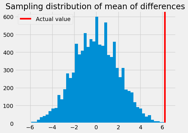
Finally we ask how unusual the actual value is in the sampling distribution from the null world:

p = np.count_nonzero(results >= actual_mean_diff) / 10000
p

0.0004

We have found that there is less than a 0.1% chance we would see the actual value, or greater, in the null world. The actual value is surprising in the null world, and we have reason to continue to investigate causes of this value, including the presumed cause, that mosquitoes are, in fact, attracted to people who drink beer.