Selecting rows from DataFrames

# Load the Pandas data science library, call it 'pd'
import pandas as pd
# Turn on a setting to use Pandas more safely.
# We will discuss this setting later.
pd.set_option('mode.copy_on_write', True)

# Load the library for plotting, name it 'plt'
import matplotlib.pyplot as plt
# Make plots look a little more fancy
plt.style.use('fivethirtyeight')

We return again to the DataFrame we were working on in basic column indexing.

# Original data frame before dropping missing values.
gender_data = pd.read_csv('gender_stats_min.csv')
labeled_gdata = gender_data.dropna().set_index('country_code')
# Show the result
labeled_gdata

	country_name	gdp_us_billion	mat_mort_ratio	population
country_code
AFG	Afghanistan	19.961015	444.00	32.715838
AGO	Angola	111.936542	501.25	26.937545
ALB	Albania	12.327586	29.25	2.888280
ARE	United Arab Emirates	375.027082	6.00	9.080299
ARG	Argentina	550.980968	53.75	42.976675
...	...	...	...	...
WSM	Samoa	0.799887	54.75	0.192225
YEM	Yemen, Rep.	36.819337	399.75	26.246608
ZAF	South Africa	345.209888	143.75	54.177209
ZMB	Zambia	24.280990	233.75	15.633220
ZWE	Zimbabwe	15.495514	398.00	15.420964

179 rows × 4 columns

Thus far we have used DataFrame indexing to select columns from DataFrames.

Remember, indexing is where we use square brackets following a value in order to select data from inside that value.

We also often want to select rows from DataFrames. You have already seen the .head and .tail methods, for selecting rows.

This page covers a more general, and more useful way of selecting rows, using direct indexing with a Boolean Series (DIBS).

Direct indexing with a Boolean Series

We often want to select rows from the data frame that match some criterion.

For example, let us return to the problem of comparing richer and poorer countries. So far we have sorted the DataFrame with .sort_values and then selected the first \(n\) or last \(n\) values, using .head and .tail. But what if we wanted to select the rows corresponding the countries with a GDP above some threshold.

Here’s are the GDP values as a Series. We are using direct indexing with column labels (DICL) on the DataFrame, to get the column as a Series:

# Direct indexing with column labels (DICL).
gdp = labeled_gdata['gdp_us_billion']
gdp

country_code
AFG     19.961015
AGO    111.936542
ALB     12.327586
ARE    375.027082
ARG    550.980968
          ...    
WSM      0.799887
YEM     36.819337
ZAF    345.209888
ZMB     24.280990
ZWE     15.495514
Name: gdp_us_billion, Length: 179, dtype: float64

Here’s the histogram of GDP again:

plt.hist(gdp)

(array([169.,   6.,   2.,   0.,   0.,   1.,   0.,   0.,   0.,   1.]),
 array([1.77430636e-01, 1.73707215e+03, 3.47396686e+03, 5.21086158e+03,
        6.94775630e+03, 8.68465102e+03, 1.04215457e+04, 1.21584404e+04,
        1.38953352e+04, 1.56322299e+04, 1.73691246e+04]),
 <BarContainer object of 10 artists>)

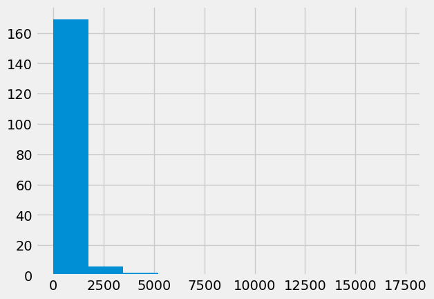
Looking at the histogram, we could try 1000 (billion US dollars) as a threshold to identify high GDP countries.

As you have found in the Series are like arrays page, Series are like arrays in many ways. As you remember, if you do a comparison on an array, you get a Boolean array, where each value in the Boolean array is the True or False answer to the comparison question for the corresponding element in the original array. If you do a comparison on a Series, you get a Boolean Series, where each value in the Series is the True or False answer to the comparison question for the corresponding element in the original Series.

For example, here we do a comparison on the gdp series, and we get a Boolean Series.

gdp_gt_1000 = gdp > 1000
gdp_gt_1000

country_code
AFG    False
AGO    False
ALB    False
ARE    False
ARG    False
       ...  
WSM    False
YEM    False
ZAF    False
ZMB    False
ZWE    False
Name: gdp_us_billion, Length: 179, dtype: bool

Notice that the Boolean Series has the same row labels (index) as the original Series (here, gdp).

The Boolean Series is — a Series:

type(gdp_gt_1000)

pandas.core.series.Series

We can use this Boolean series to select rows from the DataFrame, by Boolean indexing — direct indexing with Boolean Series (DIBS).

When we index using the Boolean Series inside the square brackets, it works like as it does when we index an array with a Boolean array:

rich_gender_data = labeled_gdata[gdp_gt_1000]
rich_gender_data

	country_name	gdp_us_billion	mat_mort_ratio	population
country_code
AUS	Australia	1422.994116	6.00	23.444560
BRA	Brazil	2198.765606	49.50	204.159544
CAN	Canada	1708.473627	7.25	35.517119
CHN	China	10182.790479	28.75	1364.446000
DEU	Germany	3601.226158	6.25	81.281645
ESP	Spain	1299.724261	5.00	46.553128
FRA	France	2647.649725	8.75	66.302099
GBR	United Kingdom	2768.864417	9.25	64.641557
IND	India	2019.005411	185.25	1293.742537
ITA	Italy	2005.983980	4.00	60.378795
JPN	Japan	5106.024760	5.75	127.297102
KOR	Korea, Rep.	1346.751162	12.00	50.727212
MEX	Mexico	1188.802780	40.00	124.203450
RUS	Russian Federation	1822.691700	25.25	143.793504
USA	United States	17369.124600	14.00	318.558175

type(rich_gender_data)

pandas.core.frame.DataFrame

rich_gender_data is a new data frame, that is a subset of the original labeled_gdata frame. It contains only the rows where the GDP value is greater than 1000 billion dollars. Check the display of rich_gender_data above to confirm that the values in the gdp_us_billion column are all greater than 1000.

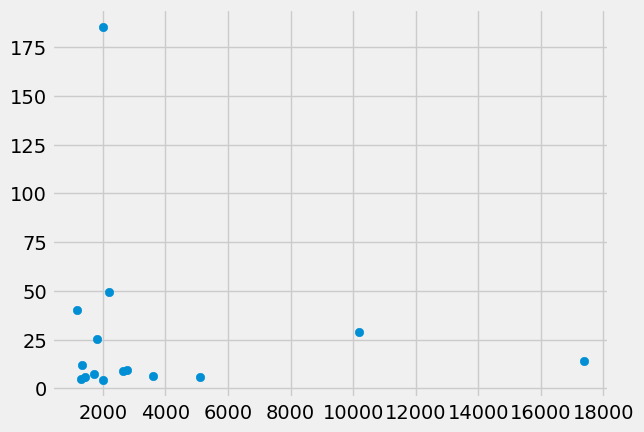
We can do a scatter plot of GDP values against maternal mortality rate, and we find again that, for rich countries, there is little relationship between GDP and maternal mortality.

plt.scatter(rich_gender_data['gdp_us_billion'],
            rich_gender_data['mat_mort_ratio'])

<matplotlib.collections.PathCollection at 0x753ddfb4f090>