The meaning of the mean

The mean is an interesting value.

In this notebook, we fetch an example sequence of numbers, with a distribution that is far from the standard bell-curve distribution. We look at the properties of the mean as a predictor of the whole distribution.

First we load our usual libraries.

import numpy as np
# Make random number generator.
rng = np.random.default_rng()
import matplotlib.pyplot as plt
# Make plots look a little bit more fancy
plt.style.use('fivethirtyeight')
# Print to 2 decimal places, show tiny values as 0
np.set_printoptions(precision=2, suppress=True)

We need Pandas to load the gender data that we first saw in the data frame introduction.

import pandas as pd
pd.set_option('mode.copy_on_write', True)

The dataset is gender_stats.csv. This contains some World Bank statistics for each country on health and economic factors related to gender equality. See the data file page for more detail.

# Load the data file
gender_data = pd.read_csv('gender_stats.csv')

In this case, we are only interested in the data for the Maternal Mortality Ratio mat_mort_ratio.

mat_mort_ratio = gender_data['mat_mort_ratio']

There are many NaN values in mat_mort_ratio. For simplicity, we drop these.

mat_mort_valid = mat_mort_ratio.dropna()

mat_mort_valid is a still a Pandas Series:

type(mat_mort_valid)

pandas.core.series.Series

Again, to make things a bit simpler, we convert this Series to an ordinary Numpy array:

mm_arr = np.array(mat_mort_valid)

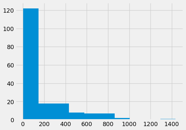
The values for mm_arr are very far from a standard bell-curve or normal distribution.

plt.hist(mm_arr);

We are interested in the mean.

mm_mean = np.mean(mm_arr)
mm_mean

175.724043715847

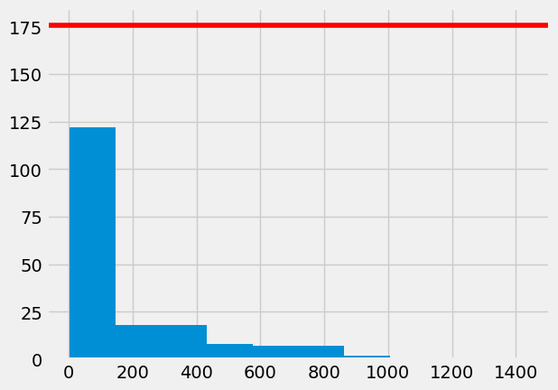
Plot the mean position on the histogram:

plt.hist(mm_arr);
plt.axhline(mm_mean, color='red')

<matplotlib.lines.Line2D at 0x747c94b74950>

As you remember, we get the mean by adding up all the values, and then dividing by the number of values, often written as \(n\).

np.sum(mm_arr) / len(mm_arr)

175.724043715847

Guess the center game

Now let’s consider the following game.

Your job is to guess the center value of an array of values. Here we’ve been working on mm_arr, but it could be any array.

You don’t know anything at all about these values, but I have all the values in front of me.

For example, let’s say the values are:

secret_values = np.array([10, 3, -7, -12, 99, 23])

I will give you £10, then ask you to make your guess.

I will take away some money if your guess for the center value is not good.

What is a good center value? We will define a good center value as being a value where I get a small sum of deviations.

The deviations are the values I get when I subtract your guess from the array of values.

Let’s say your guess was 10:

your_guess = 10

The deviations are:

# Subtract your guess from all the values in secret_values
secret_deviations = secret_values - your_guess
secret_deviations

array([  0,  -7, -17, -22,  89,  13])

The sum of the deviations is the result of adding up all the deviations.

sum_deviations = np.sum(secret_deviations)

The sum of deviations is small when the absolute value of sum of of deviations is close to 0.

abs_sum_dev = np.abs(sum_deviations)
abs_sum_dev

56

When you give my your guess your_guess, I will calculate abs_sum_dev, and ask you for that much money back.

Let’s put the calculation together into a function I will run, to tell you the money you need to pay:

def money_you_pay(values_array, guess):
    """ Give the absolute of the sum of devations

    Parameters
    ----------
    values_array : array
        An array of values that I know and you do not.
    guess : float
        A single number that is your guess for the center
        of the spread of `values_array`

    Returns
    -------
    you_pay : float
        The absolute value of the sum of deviations.
    """
    deviations = values_array - guess
    return np.abs(np.sum(deviations))

The function just repeats the calculation we did above:

money_you_pay(secret_values, your_guess)

56

So far you are at a disadvantage, because you don’t know anything about the numbers in secret_array. They could all be more than a million, so if your_guess is 10, you will lose a lot of money.

To make it fair, I will allow you to ask me for the result of one calculation on secret_numbers. It can be anything — you could ask for the median, the mode, the mean, a random element from the array, or anything else.

What number would you ask for, to help you give a good guess?

The mean as a predictor

Now let’s say that you asked me to calculate the mean, and you used that as your guess.

Let’s try that on secret_values:

money_you_pay(secret_values, np.mean(secret_values))

1.0658141036401503e-14

Nice! The money you pay is very close to 0 - and you win (near as dammit) £10!

Now let’s imagine the secret values are in fact the MMR values — mm_arr.

money_you_pay(mm_arr, np.mean(mm_arr))

2.2737367544323206e-12

Nice again!

You win, because the sum of deviations adds up to (very_nearly) 0.

mm_mean = np.mean(mm_arr)
# Sum of deviations from the mean.
np.sum(mm_arr - mm_mean)

2.2737367544323206e-12

In fact, this is a property of the mean. The deviations from the mean sum to zero.

In fact, it is not very hard to show that the deviations must sum to zero.

Sum of squared deviations

Another prediction we might be interested in, is one that gives us the smallest squared difference from the actual values.

Here are the squared differences from the mean.

# Squared prediction errors, for the mean
deviations = mm_arr - mm_mean
sq_deviations = deviations ** 2
# Show the first ten
sq_deviations[:10]

array([ 71971.99, 105967.15,  21454.65,  28806.25,  14877.67,  22044.54,
        28806.25,  29489.15,  22642.44, 326641.92])

Call the deviations — the prediction errors. They are errors because the deviation is the distance of the prediction (here, mm_mean) from the actual value.

With a good prediction (guess), we might want these squared prediction errors (squared deviations) to be small. We can see how small these are by adding them all up. This gives us the sum of squares or sum of squared error.

sos = np.sum(sq_deviations)
sos

10611707.56420765

The value above is the sum of squared prediction errors when we use the mean as the predictor. Could some other value give us a better (lower) sum of squared prediction error?

Let’s try lots of predictors, to see which gives us the smallest squared prediction error.

# Try lots of values between 150 and 210
predictors = np.arange(150, 210, 0.1)
# First 10
predictors[:10]

array([150. , 150.1, 150.2, 150.3, 150.4, 150.5, 150.6, 150.7, 150.8,
       150.9])

We make a function that accepts the values, and the predictor as arguments, and returns the sum of squares of the prediction errors:

def sum_of_squares(vals, predictor):
    deviations = vals - predictor
    sq_deviations = deviations ** 2
    return np.sum(sq_deviations)

We confirm that this gives us the value we saw before, when we use the mean as a predictor:

sum_of_squares(mm_arr, mm_mean)

10611707.56420765

Here’s what we get if we use the first predictor value:

sum_of_squares(mm_arr, predictors[0])

10732803.5

Now we try all the predictor values, to see which value gives us the lowest sum of squared errors.

# How many predictors do we have to try?
n_predictors = len(predictors)
n_predictors

600

# An array to store the sum of squares values for each predictor
sos_for_predictors = np.zeros(n_predictors)

We calculate all the sums of squares:

for i in np.arange(n_predictors):
    predictor = predictors[i]
    sos = sum_of_squares(mm_arr, predictor)
    sos_for_predictors[i] = sos

Which predictor is giving us the lowest value for the sum of squares?

plt.plot(predictors, sos_for_predictors)
plt.xlabel('Predictor')
plt.ylabel('Sum of squares');

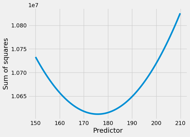
The smallest value we found for the sum of squares was:

np.min(sos_for_predictors)

10611707.67

In fact, the value for the mean is even lower:

sum_of_squares(mm_arr, mm_mean)

10611707.56420765

Plot the position of the mean on the plot of sum of squares:

plt.plot(predictors, sos_for_predictors)
plt.axhline(mm_mean, color='red')
plt.xlabel('Predictor')
plt.ylabel('Sum of squares');

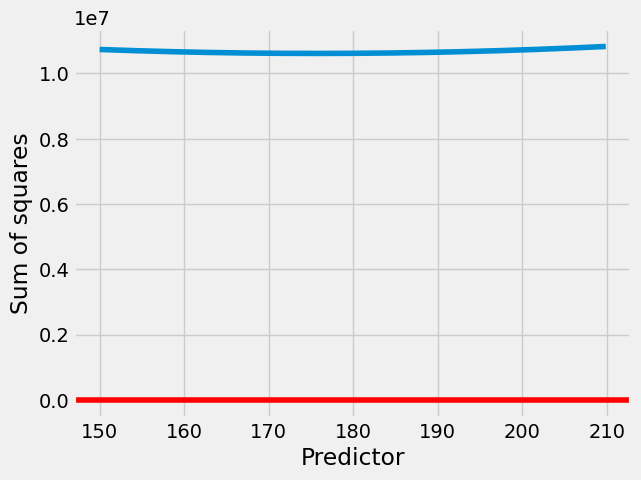
We would have to use some fairly simple calculus and algebra to show this, but the mean has to give the lowest sum of squares error.

Put another way, the mean minimizes:

• the sum of the deviations (errors);

• the sum of squared deviations (errors).