Chi-squared and the lady tasting tea#
Here we return for another analysis of the lady tasting tea.
As you remember, Muriel Bristol was sure she could taste the difference between tea where the milk was poured before the tea (milk-first), and tea where the tea was poured before the milk.
Fisher didn’t believe her, so they ended up with an experiment where Muriel got 8 cups of tea, four with milk-first, and four with milk-second. She had to choose the 4 milk-first cups, and she got them all right.
import numpy as np
# A numpy random number generator
rng = np.random.default_rng()

import pandas as pd
# Safe setting for Pandas.  Needs Pandas version >= 1.5.
pd.set_option('mode.copy_on_write', True)

# Load the library for plotting, name it 'plt'
import matplotlib.pyplot as plt
# Make plots look a little more fancy
plt.style.use('fivethirtyeight')
We reconstruct something like the experimental data.
# Whether the milk went into the cup first.
milk_first = np.repeat(['yes', 'no'], [4, 4])
# Muriel's identifications were all correct.
says_milk_first = np.repeat(['yes', 'no'], [4, 4])
tea_df = pd.DataFrame()
tea_df['milk_first'] = milk_first
tea_df['says_milk_first'] = says_milk_first
# Fisher randomized the order.   We'll just make any random order.
tea_df = tea_df.sample(8).reset_index(drop=True)
tea_df
| milk_first | says_milk_first | |
|---|---|---|
| 0 | no | no |
| 1 | no | no |
| 2 | yes | yes |
| 3 | yes | yes |
| 4 | no | no |
| 5 | no | no |
| 6 | yes | yes |
| 7 | yes | yes |
This gave us the following cross-tabulation:
tea_counts = pd.crosstab(tea_df['milk_first'], tea_df['says_milk_first'])
tea_counts
| says_milk_first | no | yes |
|---|---|---|
| milk_first | ||
| no | 4 | 0 |
| yes | 0 | 4 |
In what follows, we will refer to this DataFrame as the counts table, because it is the result of the cross-tabulation function.
In fact we will refer to this particular counts table as the observed counts table, because it has the counts that we saw in the real world, where Muriel identified the cups in Fisher’s experiment.
observed_counts = tea_counts
observed_counts
| says_milk_first | no | yes |
|---|---|---|
| milk_first | ||
| no | 4 | 0 |
| yes | 0 | 4 |
The sum over the rows give us the total counts of Muriels “no” and of Muriel’s “yes” answers. These are the column totals:
# Sum over the rows (one sum per column)
column_totals = observed_counts.sum(axis='index')
In fact, summing over the rows is the default:
observed_counts.sum()
says_milk_first
no     4
yes    4
dtype: int64
Summing over the columns gives the row totals, one sum per row. These are the total number of “yes” and “no” for milk-first:
row_totals = observed_counts.sum(axis='columns')
row_totals
milk_first
no     4
yes    4
dtype: int64
As usual, we wanted to know whether we could get evidence against the null-model, in which Muriel was choosing randomly.
As usual, to do this, we had to select a statistic that represented the effect we were interested in.
In the Lady tasting tea page, we decided to use Muriel’s number correct - 8 cups out of 8.
We simulated the null-world by shuffling Muriel’s answers (in tea_df['say_milk_first']) to be random, and recalculating the statistic (the number correct). We looked at the distribution of this statistic in the null-world, and compared the observed real-world statistic to the null-world distribution.
Now let’s consider another statistic, instead of the number correct.
The statistic is called chi-squared, and it is a statistic we can calculate from the counts table.
Chi-squared is two things#
Chi-squared can refer to two things:
The chi-squared statistic
The chi-squared test, a mathematical test that uses the chi-squared statistic to calculate a probability value.
Note - we sometimes write chi-squared as \(\chi^2\), using the Greek letter chi (pronounced to rhyme with “pie”).
The chi-squared statistic is a statistic we can calculate from
any given counts table. It is a measure of how far the table is
from the table we expect when there is a random association
between the categories — in our case, between milk_first “yes”
/”no” and Muriel’s decision “yes” / “no”.
The chi-squared test is a particular mathematical procedure to calculate a probability value from a given chi-squared statistic, without doing thousands of simulation trials.
We could use the chi-squared statistic as the statistic to calculate on a real observed counts table, and then shuffle the labels, as we have done above, to find the distribution of the chi-squared value in the null-world. This is what we do below. Or you could use the mathematical techniques embedded in the chi-squared test to generate a probability value. The two values will usually be very similar, and have the same interpretation. See below for discussion of when you might use the chi-squared test in preference to the randomization / simulation method you have seen so far.
The Chi-squared statistic#
The chi-squared statistic is a measure of how far the counts table deviates from the counts table we would expect, if the relationship between the two observation columns is random.
What does this mean in our case? The expected table is the table we expect when Muriel cannot tell whether the cup is milk-first or not.
We have already done our simulation to estimate the distribution of correct counts when Muriel is guessing, but let’s go back and get the distribution of each cell when Muriel is guessing. In the next cell, we follow the same procedure as before, shuffling Muriel’s ‘yes’ and ‘no’ answers randomly so they have a random relationship to the actual ‘yes’ and ‘no’ for milk first. This time we will look at the answers we get for a single cell of the counts table, the “yes”, “yes” cell.
Here is one trial, where we permute and rebuild the counts table:
fake_says = rng.permutation(says_milk_first)
fake_counts = pd.crosstab(milk_first, fake_says)
fake_counts
| col_0 | no | yes |
|---|---|---|
| row_0 | ||
| no | 2 | 2 |
| yes | 2 | 2 |
Because the total number of “yes” and “no” labels have not changed, the column totals and the row totals cannot change:
# In fact, axis='index' is the default.  Sum downwards.
column_totals = fake_counts.sum(axis='index')
column_totals
col_0
no     4
yes    4
dtype: int64
# Sum left to right.
row_totals = fake_counts.sum(axis='columns')
row_totals
row_0
no     4
yes    4
dtype: int64
In particular, we want the “yes”, “yes” cell of that table:
fake_counts.loc['yes', 'yes']
2
Now we know how to do one trial, we can extend to 1000 trials:
n_iters = 1000
# Make array of *integers* to store counts for each trial.
fake_yes_yes = np.zeros(n_iters, dtype=int)
for i in np.arange(n_iters):
    fake_says = rng.permutation(says_milk_first)
    fake_counts = pd.crosstab(milk_first, fake_says)
    fake_yes_yes[i] = fake_counts.loc['yes', 'yes']
fake_yes_yes[:10]
array([2, 3, 2, 3, 2, 0, 3, 1, 2, 1])
plt.hist(fake_yes_yes, bins=np.arange(6));

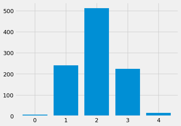
In this case the histogram is a little difficult to read, because the x-axis labels. The first bar goes from x=0 to x=1, but in fact the height is for all values equal to 0. Likewise the 1 to 2 bar refers to values equal to 1. We will use a simple routine that counts the number of 0s, 1s, 2s … and then plots those counts as a bar graph, to make the meaning of the x-axis and bars more clear.
The main engine for the function below is np.bincount. This takes an array of integers, and counts the number of 0s, the number of 1s, 2s, 3s etc. The array that comes back has the counts of 0s at position 0, the count of 1 at position 1, and so on.
We could do this the long way round like this:
print('Count of 0s:', np.count_nonzero(fake_yes_yes == 0))
print('Count of 1s:', np.count_nonzero(fake_yes_yes == 1))
print('Count of 2s:', np.count_nonzero(fake_yes_yes == 2))
print('Count of 3s:', np.count_nonzero(fake_yes_yes == 3))
print('Count of 4s:', np.count_nonzero(fake_yes_yes == 4))
Count of 0s: 7
Count of 1s: 241
Count of 2s: 512
Count of 3s: 224
Count of 4s: 16
np.bincount does this job for us:
counts_of_counts = np.bincount(fake_yes_yes)
counts_of_counts
array([ 7, 241, 512, 224, 16])
counts_of_counts[2]
512
Notice that the array is of length 5, because the largest value that Numpy found was 5, with the count stored at position 5.
We can use np.bincount to make a nice-looking plot of the counts, that is a bit clearer than the standard histogram:
def plot_int_counts(arr):
    """ Do bar plot of counts for integers in `arr`
    """
    # Convert arr to integers if necessary.
    to_count = arr.astype(int)
    # Counts for each integer in to_count
    counts = np.bincount(arr)
    # Do bar graph with integer on x axis, counts on y.
    x_vals = np.arange(len(counts))
    plt.bar(x_vals, counts)
    plt.xticks(x_vals)
plot_int_counts(fake_yes_yes)
The average value is:
np.mean(fake_yes_yes)
2.001
In fact, if you do the same thing for all four cells of the table, you’ll find the average value will be close to 2. And in fact, the average value if we take an enormous number of trials will get closer and closer to 2.
The expected value is the average value in the long run — if we do an infinite number of trials.
Note — this is actually a technical term in statistics. The expectation of a particular value is the value of the mean in the long run.
We will find that the expected number is 2.
Expected value in a counts table#
In fact, we can work out that 2 is the expected value by looking at the row and column totals.
Let’s start with our row of interest, the yes row for milk-first:
observed_counts.loc['yes']
says_milk_first
no     0
yes    4
Name: yes, dtype: int64
We know that there must be 4 yes labels to account for, and they must be distributed between the says_milk_first: no and says_milk_first: yes columns. How should we expect them to be distributed, in the null world, where Muriel is guessing?
There are 8 cups in total:
row_totals
row_0
no     4
yes    4
dtype: int64
n_total = row_totals.sum()
n_total
8
To get the proportion of says_milk_first no and yes , we need the column totals:
column_totals
col_0
no     4
yes    4
dtype: int64
Muriel is choosing 4 no and 4 yes cups, out of a total of 8.
Overall, when she is guessing for any particular cup, she has a 4 / 8 chance of guessing no and a 4 / 8 chance of guessing yes:
col_proportions = column_totals / n_total
col_proportions
col_0
no     0.5
yes    0.5
dtype: float64
Returning to our milk_first, yes row, we expect then, that of the 4 cups in this row, 0.5 * 4 will be no and 0.5 * 4 will be no:
expected_milk_first_yes = row_totals.loc['yes'] * col_proportions
expected_milk_first_yes
col_0
no     2.0
yes    2.0
dtype: float64
Observed, expected, chi-squared#
Here then is the counts table with the expected values (the values we expect in the long run, if the association between the actual “yes”, “no” of milk-first, and Muriel’s answers.
expected_counts = pd.DataFrame([[2, 2], [2, 2]],
                               index=['no', 'yes'],
                               columns=['no', 'yes'])
expected_counts
| no | yes | |
|---|---|---|
| no | 2 | 2 |
| yes | 2 | 2 |
The Scipy chi-squared routine will calculate that expected table for us, as an array:
import scipy.stats as sps

# Basic chi-squared calculation, turning off correction.
observed_stat, p_value, dof, exp_array = sps.chi2_contingency(
    observed_counts, correction=False)
exp_array
array([[2., 2.],
       [2., 2.]])
We can then look at how much the expected counts differ from the actual counts we saw in the real world. We could go through subtracting the entries in the expected counts table from the entries in the observed counts table, one by one, but Pandas is clever enough to understand this is what we want when we subtract the two DataFrames directly:
obs_minus_exp = observed_counts - expected_counts
obs_minus_exp
| says_milk_first | no | yes |
|---|---|---|
| milk_first | ||
| no | 2 | -2 |
| yes | -2 | 2 |
In textbooks, you will often see the observed values written as “O” (capital “o”) and the expected values written as “E”:
O = observed_counts
E = expected_counts
O_minus_E = O - E
O_minus_E
| says_milk_first | no | yes |
|---|---|---|
| milk_first | ||
| no | 2 | -2 |
| yes | -2 | 2 |
The observed minus expected table shows us how far each entry in the table was from the expected value. Call this the deviations table.
We would like an overall measure of how far the observed table was from the expected table. We could just add up all the values in the deviation table, like this:
# Sum over the rows, and then take the sum of sums.
(O - E).sum().sum()
0
This isn’t very helpful, because the positive and negative deviations from the expected values are cancelling each other out. In order to avoid this, we can make all the differences positive, by squaring them:
(O - E) ** 2
| says_milk_first | no | yes |
|---|---|---|
| milk_first | ||
| no | 4 | 4 |
| yes | 4 | 4 |
In our case, the expected values are all the same, because the total numbers in the rows and columns are all the same, but that is rarely the case. When there are small numbers over the row or the column or both, the expected number will also be small, and we may want to take that into account by dividing the squared deviations by the expected values, to give a squared deviation as a proportion of expected, the proportional squared deviation:
(O - E) ** 2 / E
| says_milk_first | no | yes |
|---|---|---|
| milk_first | ||
| no | 2.0 | 2.0 |
| yes | 2.0 | 2.0 |
We can now take an overall measure of how far the table is from expected, by summing up the values in this proportional squared deviation table, to get the chi-squared statistic:
chi_squared = ((O - E) ** 2 / E).sum().sum()
chi_squared
8.0
This is exactly the statistic that the Scipy chi-squared routine calculates for us, along with the expected table:
# Basic chi-squared calculation, turning off correction.
observed_stat, p_value, dof, exp_array = sps.chi2_contingency(
    observed_counts, correction=False)
exp_array
array([[2., 2.],
       [2., 2.]])
observed_stat
8.0
Testing chi-squared with simulation#
Notice that we have just calculated the chi-squared statistic — a statistic we can calculate on a particular counts table.
Notice too that the expected table E cannot not change for
any permutation of Muriel’s “yes” / “no” answers, because the
total number of milk_first “yes” and “no”, or Muriel’s “yes”
and “no”, cannot change. This is the same as saying that the row
and column totals cannot change. The expected table E depends
only on the row and column totals.
We can use our column permutation method to make many counts table from the null-world, and calculate chi-squared values on these:
# One trial in the null-world, chi-squared on the fake table.
fake_says = rng.permutation(says_milk_first)
fake_O = pd.crosstab(milk_first, fake_says)
fake_chi2 = ((fake_O - E) ** 2 / E).sum().sum()
fake_chi2
0.0
n_iters = 1000
fake_chi2_vals = np.zeros(n_iters)
for i in np.arange(n_iters):
    fake_says = rng.permutation(says_milk_first)
    fake_O = pd.crosstab(milk_first, fake_says)
    fake_chi2_vals[i] = ((fake_O - E) ** 2 / E).sum().sum()
fake_chi2_vals[:10]
array([2., 8., 2., 0., 0., 2., 0., 0., 0., 2.])
plt.hist(fake_chi2_vals);
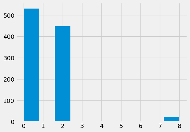
This gives our usual simulation probability of our observed chi-squared:
p_simulation = np.count_nonzero(fake_chi2_vals >= observed_stat) / n_iters
p_simulation
0.021
The traditional chi-squared test#
It turns out that we can also use a mathematical technique to calculate a probability of seeing a chi-squared value as large or larger, on the assumption that the relationship between the cross-tabulated labels is actually random. The details of this involve a lot more mathematics than we can go into in this course. It is this probability value that comes back from Scipy:
# Basic chi-squared calculation, turning off correction.
observed_stat, p_value, dof, exp_array = sps.chi2_contingency(
    observed_counts, correction=False)
p_value
0.004677734981047276
As you can see, this probability value is a lot smaller than the one we calculated using simulation, and that is because we have unwisely turned off the necessary correction for 2 by 2 tables in the Scipy routine:
# chi-squared calculation with Yates correction for 2x2 tables
corr_stat, corr_p_value, dof, exp_array = sps.chi2_contingency(
    observed_counts, correction=True)
corr_p_value
0.033894853524689295
Notice that the mathematical value is very similar to our familiar simulation value.
The expected values#
We made our lives easier in the example above, by having the same number of “yes” and “no” labels for each of the two categories (milk-first, and says-milk-first).
But — what if there are not the same number of labels in the two categories? What are the expected values in that case.
Let’s imagine an experiment like Fisher’s, but where only two of the tea-cups had milk poured first. Muriel knows there are only two, and chooses two of the eight cups. Let’s imagine that Muriel is still all-knowing when it comes to milk-first and tea:
# Whether the milk went into the cup first.
milk_first_2_6 = np.repeat(['yes', 'no'], [2, 6])
# Muriel's identifications were all correct.
says_milk_first_2_6 = np.repeat(['yes', 'no'], [2, 6])
tea_df_2_6 = pd.DataFrame()
tea_df_2_6['milk_first'] = milk_first_2_6
tea_df_2_6['says_milk_first'] = says_milk_first_2_6
tea_df_2_6 = tea_df_2_6.sample(8).reset_index(drop=True)
tea_df_2_6
| milk_first | says_milk_first | |
|---|---|---|
| 0 | yes | yes |
| 1 | no | no |
| 2 | no | no |
| 3 | no | no |
| 4 | yes | yes |
| 5 | no | no |
| 6 | no | no |
| 7 | no | no |
The observed counts table in this case is:
observed_counts_2_6 = pd.crosstab(milk_first_2_6,
                                  says_milk_first_2_6)
observed_counts_2_6
| col_0 | no | yes |
|---|---|---|
| row_0 | ||
| no | 6 | 0 |
| yes | 0 | 2 |
Let’s do the same test as before, where our statistic of interest is the yes, yes value.
observed_statistic_2_6 = observed_counts_2_6.loc['yes', 'yes']
observed_statistic_2_6
2
What is the distribution and expected value of this statistic, in the null-world?
n_iters = 1000
fake_yes_yes_2_6 = np.zeros(n_iters, dtype=int)
for i in np.arange(n_iters):
    fake_says_2_6 = rng.permutation(says_milk_first_2_6)
    fake_counts_2_6 = pd.crosstab(milk_first_2_6, fake_says_2_6)
    fake_yes_yes_2_6[i] = fake_counts_2_6.loc['yes', 'yes']
fake_yes_yes_2_6[:10]
array([0, 0, 0, 0, 0, 0, 2, 1, 0, 1])
plot_int_counts(fake_yes_yes_2_6)
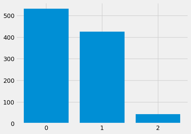
In the null-world, the average count for the yes, yes entry is around 0.5:
np.mean(fake_yes_yes_2_6)
0.511
We speculate, that the expected value for yes, yes, in the null-world, is 0.5.
We can work out the expected value using the same logic as before.
We concentrate on our row of interest:
observed_counts_2_6
| col_0 | no | yes |
|---|---|---|
| row_0 | ||
| no | 6 | 0 |
| yes | 0 | 2 |
There must always be 2 yes labels in this row (2 cups with milk-first) to distribute between the 2 values (columns) (Muriel says no, Muriel says yes):
row_totals = observed_counts_2_6.sum(axis='columns')
row_totals
row_0
no     6
yes    2
dtype: int64
Muriel must distribute her guesses (in the null-world) as 6 no and 2 yes:
col_totals = observed_counts_2_6.sum(axis='index')
col_totals
col_0
no     6
yes    2
dtype: int64
Therefore, for any one cup, her chances of guessing no are 6/8, and of guessing yes are 2/8:
p_guess = col_totals / col_totals.sum()
p_guess
col_0
no     0.75
yes    0.25
dtype: float64
We distribute Muriel’s guesses to the expected row accordingly:
expected_row = row_totals.loc['yes'] * p_guess
expected_row
col_0
no     1.5
yes    0.5
dtype: float64
Following the same logic, we compile our new expected counts table:
E_2_6 = pd.DataFrame([[6 * 6 / 8, 6 * 2 / 8],
                      [2 * 6 / 8, 2 * 2 / 8]],
                     index=['no', 'yes'],
                     columns=['no', 'yes'])
E_2_6
| no | yes | |
|---|---|---|
| no | 4.5 | 1.5 |
| yes | 1.5 | 0.5 |
# Chi-squared
O_2_6 = observed_counts_2_6
((O_2_6 - E_2_6) ** 2 / E_2_6).sum().sum()
8.0
As before, this is the expected table and statistic that Scipy calculates for us.
obs_stat_2_6, p_value_2_6, dof, exp_array_2_6 = sps.chi2_contingency(
    observed_counts_2_6, correction=False)
exp_array_2_6
array([[4.5, 1.5],
       [1.5, 0.5]])
obs_stat_2_6
8.0
Chi-squared statistics and tests#
Summary:
First — choose your statistic of interest. You might be interested in a particular entry in your counts table, or the chi-squared measure of deviation from expected, or something else.
When testing, and using a measure that isn’t chi-squared, you will want to use simulation to work out how unusual your observed statistic is.
If you are using the chi-squared statistic you might consider using simulation for testing, or the mathematical method implemented in — for example — Scipy.
In the old days, using simulation was not common, and you would likely be using the chi-squared mathematical test in this situation. Then, as now, if you are using the mathematical testing method, you would need to know some rules about when to use particular tests. The rules were something like:
Calculate the expected counts. If the minimum of the expected counts is less than 5, use the Fisher exact test.
Otherwise, use the Chi-square test.
For a 2 by 2 table, apply the Yates correction (
correction=True) above.
Now you have resampling (AKA simulation), you can just choose your statistic and calculate your sampling distribution, in order to get your p-value.