Introducing principal component analysis

Introducing principal component analysis#

This page was much inspired by these two excellent tutorials:

Background#

Check that you understand:

Vector projection;
Matrix multiplication. See this Khan academy introduction to matrix multiplication. I highly recommend Gilbert Strang’s lecture on matrix multiplication.

Setting the scene#

Start by loading the libraries we need, and doing some configuration:

import numpy as np
import numpy.linalg as npl
# Display array values to 6 digits of precision
np.set_printoptions(precision=6, suppress=True)

import pandas as pd
pd.set_option('mode.copy_on_write', True)

import matplotlib.pyplot as plt

We are going to use the English Premier League (EPL) table data for this example. See the EPL dataset page for more on this dataset.

df = pd.read_csv('data/premier_league_2021.csv')
df.head()

	rank	team	played	won	drawn	lost	for	against	goal_difference	points	wages_year	keeper	defense	midfield	forward
0	1	Manchester City	38	29	6	3	99	26	73	93	168572	8892	60320	24500	74860
1	2	Liverpool	38	28	8	2	94	26	68	92	148772	14560	46540	47320	40352
2	3	Chelsea	38	21	11	6	76	33	43	74	187340	12480	51220	51100	72540
3	4	Tottenham Hotspur	38	22	5	11	69	40	29	71	110416	6760	29516	30680	43460
4	5	Arsenal	38	22	3	13	61	48	13	69	118074	8400	37024	27300	45350

Notice we have spending data on defense, midfield and forward. As we will see, these are highly correlated, one with another.

Our particular interest is to see whether we can extract some summary of the defense and forward spending. We suspect there is something common there, and we want to see if we can summarize it better.

While we’re at it, let’s convert the wages to units of 10 million GBPs (£), to make the numbers a bit easier to read at a glance.

data = df[['defense', 'forward']] / 10_000
data.head()

	defense	forward
0	6.0320	7.4860
1	4.6540	4.0352
2	5.1220	7.2540
3	2.9516	4.3460
4	3.7024	4.5350

We will put these numbers into a 2D Numpy array X:

X = np.array(data)
X

array([[ 6.032 ,  7.486 ],
       [ 4.654 ,  4.0352],
       [ 5.122 ,  7.254 ],
       [ 2.9516,  4.346 ],
       [ 3.7024,  4.535 ],
       [ 6.048 , 11.278 ],
       [ 2.886 ,  2.704 ],
       [ 2.804 ,  2.544 ],
       [ 1.764 ,  1.679 ],
       [ 2.0736,  2.682 ],
       [ 2.7276,  2.404 ],
       [ 2.093 ,  2.6   ],
       [ 0.8686,  0.962 ],
       [ 2.616 ,  3.647 ],
       [ 1.2137,  2.153 ],
       [ 3.1512,  3.931 ],
       [ 1.315 ,  1.8144],
       [ 1.494 ,  1.511 ],
       [ 1.488 ,  0.928 ],
       [ 1.476 ,  0.628 ]])

n_rows = len(X)
n_rows

We will call the rows samples and the columns features. In our case the samples are EPL clubs, and the features are defense and forward spending.

To make things simpler, we will subtract the mean across samples from each feature. As each feature is one column, we need to subtract the mean of each column, from each value in the column:

# Subtract mean across samples (mean of each feature)
x_mean = np.mean(X, axis=0)
X[:, 0] = X[:, 0] - x_mean[0]  # Subtract mean of defense.
X[:, 1] = X[:, 1] - x_mean[1]  # Subtract mean of forward
# The columns now have means near as dammit to 0.
np.mean(X, axis=0)

array([0., 0.])

The values for the two features (columns) in \(\mathbf{X}\) are highly correlated:

plt.scatter(X[:, 0], X[:, 1])
plt.axis('equal')
plt.xlabel('Defense (feature 1)')
plt.ylabel('Forward (feature 2)')

Text(0, 0.5, 'Forward (feature 2)')

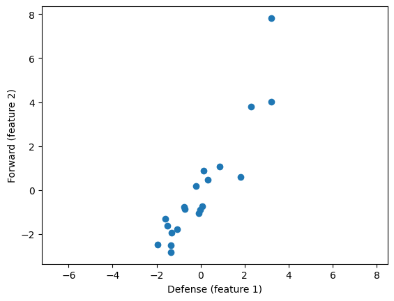
_images/a374c1441504fa06960b88e706b4b7f9bfbb1935b637a613630e488be9fb1b54.png

We want to explain the variation in these data.

The variation we want to explain is given by the sum of squares of the data values.

squares = X ** 2
print(np.sum(squares))

176.73345957749999

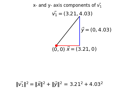
The sums of squares of the data can be thought of as the squared lengths of the 20 2D vectors in the rows of \(\mathbf{X}\).

We can think of each sample as being a point on a 2D coordinate system, where the first feature is the position on the x axis, and the second is the position on the y axis. In fact, this is how we just plotted the values in the scatter plot. We can also think of each row as a 2D vector. Call \(\vec{v_j}\) the vector contained in row \(j\) of matrix \(\mathbf{X}\), where \(j \in 1..20\).

The sum of squares across the features, is also the squared distance of the point (row) from the origin (0, 0). That is the same as saying that the sum of squares is the squared length of \(\vec{v_j}\). This can be written as \(\|\vec{v_j}\|^2\)

Take the first row / point / vector as an example (\(\vec{v_1}\)):

v1 = X[0]
v1

array([3.207965, 4.02992 ])

So, the sums of squares we are trying to explain can be expressed as the sum of the squared distance of each point from the origin, where the points (vectors) are the rows of \(\mathbf{X}\):

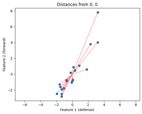
Put another way, we are trying to explain the squares of the lengths of the dotted red lines on the plot.

At the moment, we have not explained anything, so our current unexplained sum of squares is:

print(np.sum(X ** 2))

176.73345957749999

For the following you will need to know how to use vector dot products to project one vector on another.

See Vectors and dot products and Vector projection for the details, and please try the excellent Khan academy videos linked from those pages if you are new to vector dot products or are feeling rusty.

Let us now say that we want to try and find a line that will explain the maximum sum of squares in the data.

We define our line with a unit vector \(\hat{u}\). All points on the line can be expressed with \(c\hat{u}\) where \(c\) is a scalar.

Our best fitting line \(c\hat{u}\) is the line that comes closest to the points, in the sense of minimizing the squared distance between the line and points.

Put a little more formally, for each point \(\vec{v_j}\) we will find the distance \(d_j\) between \(\vec{v_j}\) and the line. We want the line with the smallest \(\sum_j{d_j^2}\).

What do we mean by the distance in this case? The distance \(d_i\) is the distance between the point \(\vec{v_i}\) and the projection of that point onto the line \(c\hat{u}\). The projection of \(\vec{v_i}\) onto the line defined by \(\hat{u}\) is, as we remember, given by \(c\hat{u}\) where \(c = \vec{v_i}\cdot\hat{u}\).

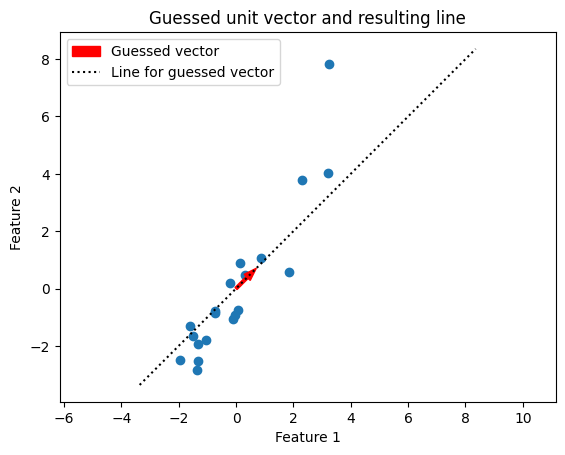
Looking at the scatter plot, we might consider trying a unit vector at 45 degrees angle to the x axis:

u_guessed = np.array([np.cos(np.pi / 4), np.sin(np.pi / 4)])
u_guessed

array([0.707107, 0.707107])

This is a unit vector:

np.sum(u_guessed ** 2)

np.float64(1.0)

Let’s project all the points onto that line:

u_col = u_guessed.reshape(2, 1)  # A column vector
c_values = X.dot(u_col)  # c values for scaling u
# Scale u by values to get projection for this guessed vector.
projected_g = c_values.dot(u_col.T)
projected_g

array([[ 3.618943,  3.618942],
       [ 1.204542,  1.204542],
       [ 3.047942,  3.047942],
       [ 0.508743,  0.508742],
       [ 0.978643,  0.978642],
       [ 5.522943,  5.522942],
       [-0.345057, -0.345057],
       [-0.466058, -0.466057],
       [-1.418557, -1.418557],
       [-0.762258, -0.762257],
       [-0.574258, -0.574257],
       [-0.793557, -0.793557],
       [-2.224757, -2.224757],
       [-0.008558, -0.008558],
       [-1.456708, -1.456707],
       [ 0.401043,  0.401042],
       [-1.575358, -1.575357],
       [-1.637558, -1.637557],
       [-1.932057, -1.932057],
       [-2.088058, -2.088057]])

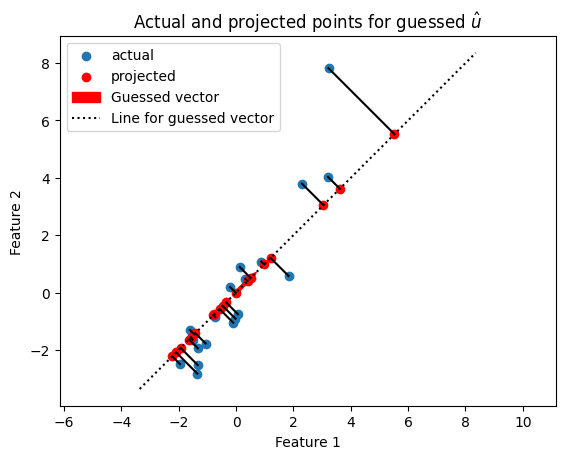
The projected points (in red), are the positions of the points that can be explained by projection onto the guessed line defined by \(\hat{u}\). The red projected points also have their own sum of squares:

print(np.sum(projected_g ** 2))

159.86964663274998

Because we are projecting onto a unit vector, \(\|c\hat{u}\|^2 = c\hat{u} \cdot c\hat{u} = c^2(\hat{u} \cdot \hat{u}) = c^2\). Therefore the c_values are also the lengths of the projected vectors, so the sum of squares of the c_values also gives us the sum of squares of the projected points:

print(np.sum(c_values ** 2))

159.86964663274998

As we will see later, this is the sum of squares from the original points that have been explained by projection onto \(\hat{u}\).

Once I have the projected points, I can calculate the remaining distance of the actual points from the projected points:

remaining_g = X - projected_g
# As-crow-flies distances between actual and projected points.
distances_g = np.sqrt(np.sum(remaining_g ** 2, axis=1))
distances_g

array([0.58121 , 0.884481, 1.060628, 0.539066, 0.141814, 3.251245,
       0.575617, 0.630771, 0.507027, 0.01672 , 0.675743, 0.08842 ,
       0.38088 , 0.282104, 0.217262, 0.104479, 0.093794, 0.434902,
       0.842903, 1.04655 ])

I can also express the overall (squared) remaining distance as the sum of squares. The following is the code version of the formula \(\sum_j{d_j^2}\) that you saw above.

print(np.sum(remaining_g ** 2))

16.86381294475001

I’m going to try a whole lot of different values for \(\hat{u}\), so I will make a function to calculate the result of projecting the data onto a line defined by a unit vector \(\hat{u}\):

def line_projection(u, X):
    """ Return columns of X projected onto line defined by u
    """
    u = u.reshape(2, 1)  # Reshape to a column vector
    c_values = X.dot(u)  # c values for scaling u
    projected = c_values.dot(u.T)
    return projected

Next a small function to return the vectors remaining after removing the projections:

def line_remaining(u, X):
    """ Return vectors remaining after removing cols of X projected onto u
    """
    projected = line_projection(u, X)
    remaining = X - projected
    return remaining

Using these little functions, I get the same answer as before:

print(np.sum(line_remaining(u_guessed, X) ** 2))

16.86381294475001

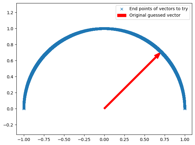
Now I will make lots of \(\hat{u}\) vectors spanning half the circle:

angles = np.linspace(0, np.pi, 10000)
n_angles = len(angles)
x = np.cos(angles)
y = np.sin(angles)
u_vectors = np.stack([x, y], axis=1)
u_vectors.shape

(10000, 2)

plt.plot(u_vectors[:, 0], u_vectors[:, 1], 'x',
         label='End points of vectors to try')
plt.arrow(0, 0, u_guessed[0], u_guessed[1], width=0.02, color='r',
          length_includes_head=True,
          label='Original guessed vector')
plt.axis('equal')
plt.tight_layout()
plt.legend();

_images/90cc4523f2b9e6615b862d54bdb64bd33d3e457d4ae547547ab4f19d6396ed37.png

I then get the remaining sum of squares after projecting onto each of these unit vectors:

remaining_ss = np.zeros(n_angles)
for i in range(n_angles):
    u = u_vectors[i]  # Get vector corresponding to angle.
    remaining = line_remaining(u, X)
    remaining_ss[i] = np.sum(remaining ** 2)
plt.plot(angles, remaining_ss)
plt.xlabel('Angle of unit vector')
plt.ylabel('Remaining sum of squares');

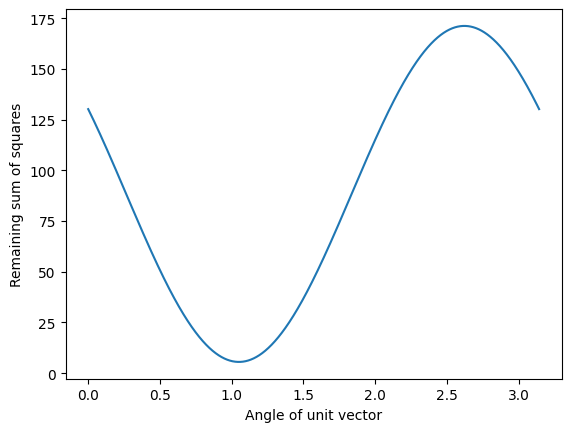
_images/7ec15d24bf64bb785190a744604a0ef4a60b2f6323195e5d19b83f6b2347abf9.png

It looks like the minimum value is for a unit vector at around angle 0.5 radians:

min_i = np.argmin(remaining_ss)
angle_best = angles[min_i]
print(angle_best)

1.0500252673564445

u_best = u_vectors[min_i]
u_best

array([0.497549, 0.867436])

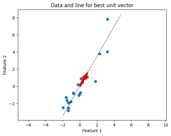
I plot the data with the new unit vector I found:

Do the projections for this best line look better than before?

projected = line_projection(u_best, X)

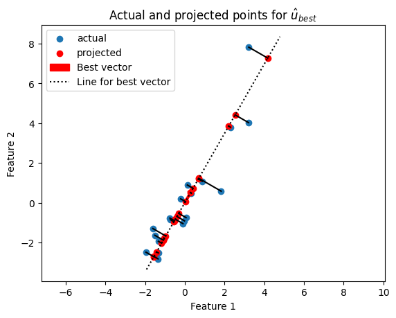
Now we have found a reasonable choice for our first best fitting line, we have a set of remaining vectors that we have not explained. These are the vectors between the projected and actual points.

remaining = X - projected

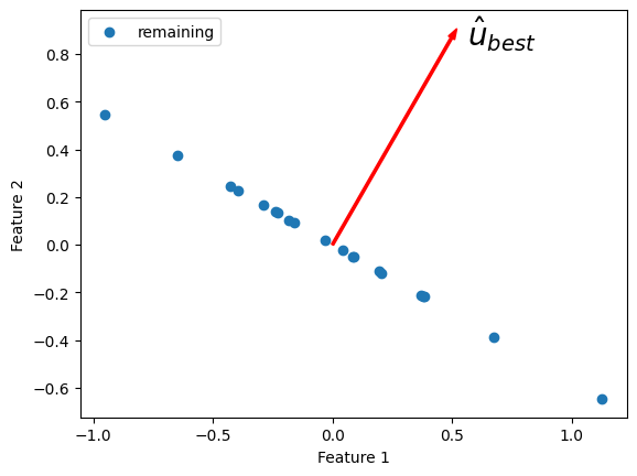
What is the next line we need to best explain the remaining sum of squares? We want another unit vector orthogonal to the first. This is because we have already explained everything that can be explained along the direction of \(\hat{u}_{best}\), and we only have two dimensions, so there is only one remaining direction along which the variation can occur.

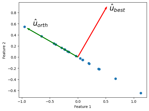
I get the new \(\hat{u}_{orth}\) vector with a rotation by 90 degrees (\(\pi / 2\)):

u_best_orth = np.array([np.cos(angle_best + np.pi / 2), np.sin(angle_best + np.pi / 2)])

Within error due to the floating point calculations, \(\hat{u}_{orth}\) is orthogonal to \(\hat{u}_{best}\):

np.allclose(u_best.dot(u_best_orth), 0)

True

The projections onto \(\hat{u}_{orth}\) are the same as the remaining points, because the remaining points already lie along the line defined by \(\hat{u}_{orth}\).

projected_onto_orth = line_projection(u_best_orth, remaining)
np.allclose(projected_onto_orth, remaining)

True

If we have really found the line \(\hat{u}_{best}\) that removes the most sum of squares from the remaining points, then this is the first principal component of \(\mathbf{X}\). \(\hat{u}_{orth}\) will be the second principal component of \(\mathbf{X}\).

Now for a trick. Remember that the two principal components are orthogonal to one another. That means, that if I project the data onto the second principal component \(\hat{u}_{orth}\), I will (by the definition of orthogonal) pick up no component of the columns of \(\mathbf{X}\) that is colinear (predictable via projection) with \(\hat{u}_{best}\).

This means that I can go straight to the projection onto the second component, from the original array \(\mathbf{X}\).

# project onto second component direct from data
projected_onto_orth_again = line_projection(u_best_orth, X)
# Gives same answer as projecting remainder from first component
np.allclose(projected_onto_orth_again, projected_onto_orth)

True

\(\newcommand{\X}{\mathbf{X}}\newcommand{\U}{\mathbf{U}}\newcommand{\S}{\mathbf{\Sigma}}\newcommand{\V}{\mathbf{V}}\newcommand{\C}{\mathbf{C}}\newcommand{\W}{\mathbf{W}}\newcommand{\Vh}{\mathbf{V*}}\) For the same reason, I can calculate the scalar projections \(c\) for both components at the same time, by doing matrix multiplication. First assemble the components into the columns of a 2 by 2 array \(\W\):

print('Best first u', u_best)
print('Best second u', u_best_orth)

Best first u [0.497549 0.867436]
Best second u [-0.867436  0.497549]

# Components as rows in a 2 by 2 array
W = np.vstack([u_best, u_best_orth])
W

array([[ 0.497549,  0.867436],
       [-0.867436,  0.497549]])

Call the 20 by 2 scalar projection values matrix \(\C\). I can calculate \(\C\) in one shot by matrix multiplication:

\[ \C = \X \W^T \]

C = X.dot(W.T)
C

array([[ 5.091817, -0.77762 ],
       [ 1.412847, -1.299236],
       [ 4.437802, -0.103685],
       [ 0.835418,  0.332124],
       [ 1.372924, -0.22511 ],
       [ 8.389094,  1.095207],
       [-0.62155 , -0.427947],
       [-0.801139, -0.436426],
       [-2.068922,  0.035328],
       [-1.044843,  0.265811],
       [-0.960593, -0.43981 ],
       [-1.10632 ,  0.208184],
       [-3.136379,  0.455287],
       [ 0.062103,  0.275449],
       [-1.931559,  0.748516],
       [ 0.574743, -0.047499],
       [-2.174871,  0.492175],
       [-2.34899 ,  0.185947],
       [-2.85769 , -0.098919],
       [-3.123891, -0.237775]])

The first column of \(\C\) has the scalar projections for the first component (the first component is the first row of \(\W\)). The second column has the scalar projections for the second component.

Finally, we can get the projections of the vectors in \(\X\) onto the components in \(\W\) by taking the dot products of the scalar projections in \(\C\) with the rows in \(\W\).

# Result of projecting on first component, via array dot
# np.outer does the equivalent of a matrix multiply of a column vector
# with a row vector, to give a matrix.
projected_onto_1 = np.outer(C[:, 0], W[0, :])
# The same as doing the original calculation
np.allclose(projected_onto_1, line_projection(u_best, X))

True

# Result of projecting on second component, via np.outer
projected_onto_2 = np.outer(C[:, 1], W[1, :])
# The same as doing the original calculation
np.allclose(projected_onto_2, line_projection(u_best_orth, X))

True

Principal components are new axes to express the data#

My original points were expressed in the orthogonal, standard x and y axes. My principal components give new orthogonal axes. When I project, I have just re-expressed my original points on these new orthogonal axes. Let’s call the projections of \(\vec{v_1}\) onto the first and second components: \(proj_1\vec{v_1}\), \(proj_2\vec{v_1}\).

For example, here is my original first point \(\vec{v_1}\) expressed using the projections onto the principal component axes:

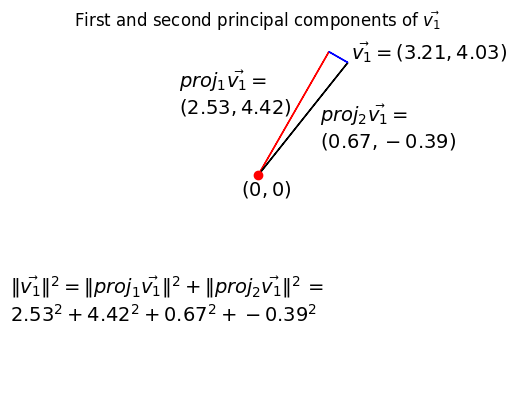
We have re-expressed \(\vec{v_1}\) by two new orthogonal vectors \(proj_1\vec{v_1}\) plus \(proj_2\vec{v_1}\). In symbols: \(\vec{v_1} = proj_1\vec{v_1} + proj_2\vec{v_1}\).

The sum of component 1 projections and the component 2 projections add up to the original vectors (points).

Sure enough, if I sum up the data projected onto the first component and the data projected onto the second, I get back the original data:

np.allclose(projected_onto_1 + projected_onto_2, X)

True

Doing the sum above is the same operation as matrix multiplication of the scalar projects \(\C\) with the components \(\W\). Seeing that this is so involves writing out a few cells of the matrix multiplication in symbols and staring at it for a while. Alternatively, you might be able to see that \(\W\) is an orthogonal matrix, and therefore, \(\W\) is the inverse of \(\W^T\). Above we have \(\C = \X \W^T\) so \(\C \W = \X\):

data_again = C.dot(W)
np.allclose(data_again, X)

True

The components partition the sums of squares#

Notice also that I have partitioned the sums of squares of the data into a part that can be explained by the first component, and a part that can be explained by the second:

# Total sum of squares
print(np.sum(X ** 2))

176.73345957749999

# Sum of squares in the projection onto the first
ss_in_first = np.sum(projected_onto_1 ** 2)
# Sum of squares in the projection onto the second
ss_in_second = np.sum(projected_onto_2 ** 2)
# They add up to the total sum of squares
print((ss_in_first, ss_in_second, ss_in_first + ss_in_second))

(np.float64(171.19843249503052), np.float64(5.535027082469528), np.float64(176.73345957750004))

Why is this?

Consider the first vector in \(\mathbf{X}\) : \(\vec{v_1}\). We have re-expressed the squared length of \(\vec{v_1}\) with the squared length of \(proj_1\vec{v_1}\) plus the squared length of \(proj_2\vec{v_1}\). The length of \(\vec{v_1}\) is unchanged, but we now have two new orthogonal vectors making up the sides of the right angled triangle of which \(\vec{v_1}\) is the hypotenuse. The total sum of squares in the data is given by:

\[\begin{split} \sum_j x^2 + \sum_j y^2 = \\ \sum_j \left( x^2 + y^2 \right) = \\ \sum_j \|\vec{v_1}\|^2 = \\ \sum_j \left( \|proj_1\vec{v_1}\|^2 + \|proj_2\vec{v_1}\|^2 \right) = \\ \sum_j \|proj_1\vec{v_1}\|^2 + \sum_j \|proj_2\vec{v_1}\|^2 \\ \end{split}\]

where \(j\) indexes samples - \(j \in 1..20\) in our case.

The first line shows the partition of the sum of squares into standard x and y coordinates, and the last line shows the partition into the first and second principal components.

Finding the principal components with SVD#

You now know what a principal component analysis is.

It turns out there is a much quicker way to find the components than the slow and dumb search that I did above.

For reasons that we don’t have space to go into, we can get the components using Singular Value Decomposition (SVD) of \(\mathbf{X}\).

See http://arxiv.org/abs/1404.1100 for more detail.

The SVD on an array containing only real (not complex) values such as \(\mathbf{X}\) is defined as:

\[ \X = \U \Sigma \V^T \]

To avoid the distraction of the transpose in the \(V^T\) notation, we will write \(\V^T\) as \(\Vh\):

\[ \X = \U \Sigma \Vh \]

If \(\X\) is shape \(M\) by \(N\) then \(\U\) is an \(M\) by \(M\) orthogonal matrix, \(\S\) is a diagonal matrix shape \(M\) by \(N\), and \(\Vh\) is an \(N\) by \(N\) orthogonal matrix.

U, S, Vstar = npl.svd(X)
U.shape, Vstar.shape

((20, 20), (2, 2))

The components are in the rows of the returned matrix \(\Vh\).

Vstar

array([[-0.49759 , -0.867412],
       [-0.867412,  0.49759 ]])

Remember that a vector \(\vec{r}\) defines the same line as the vector \(-\vec{r}\), so we do not care about a flip in the sign of the principal components:

u_best

array([0.497549, 0.867436])

u_best_orth

array([-0.867436,  0.497549])

The returned vector S gives the \(M\) singular values that form the main diagonal of the \(M\) by \(N\) diagonal matrix \(\S\). The values in S give the square root of the explained sum of squares for each component:

S ** 2

array([171.198433,   5.535027])

The formula above is for the “full” SVD. When the number of rows in \(\X\) (\(= M\)) is less than the number of columns (\(= N\)) the SVD formula above requires an \(M\) by \(N\) matrix \(\S\) padded on the right with \(N - M\) all zero columns, and an \(N\) by \(N\) matrix \(\Vh\) (often written as \(\V^T\)), where the last \(N - M\) rows will be discarded by matrix multiplication with the all zero rows in \(\S\). A variant of the full SVD is the thin SVD, where we discard the useless columns and rows and return \(\S\) as a diagonal matrix \(M x M\) and \(\Vh\) with shape \(M x N\). This is the full_matrices=False variant in NumPy:

U, S, Vstar = npl.svd(X, full_matrices=False)
U.shape, Vstar.shape

((20, 2), (2, 2))

By the definition of the SVD, \(\U\) and \(\Vh\) are orthogonal matrices, so \(\Vh^T\) is the inverse of \(\Vh\) and \(\Vh^T \V = I\). Therefore:

\[ \X = \U \Sigma \Vh \implies \X \Vh^T = \U \Sigma \]

You may recognize \(\X \Vh^T\) as the matrix of scalar projections \(\C\) above:

# Implement the formula above.
C = X.dot(Vstar.T)
np.allclose(C, U.dot(np.diag(S)))

True

Because \(\U\) is also an orthogonal matrix, it has row lengths of 1, and we can get the values in \(\S\) from the row lengths of \(\C\):

S_from_C = np.sqrt(np.sum(C ** 2, axis=0))
np.allclose(S_from_C, S)

True

S_from_C

array([13.084282,  2.352664])

Now we can reconstruct \(\U\):

# Divide out reconstructed S values
S_as_row = S_from_C.reshape((1, 2))
np.allclose(C / S_as_row, U)

True

PCA using scikit-learn#

from sklearn.decomposition import PCA

pca = PCA()
pca = pca.fit(X)

# Scikit-learn's components.
pca.components_

array([[ 0.49759 ,  0.867412],
       [ 0.867412, -0.49759 ]])

Vstar

array([[-0.49759 , -0.867412],
       [-0.867412,  0.49759 ]])

Notice the components contain the same vectors as \(\Vh\) above, with the components in the rows - but where the components can have their signs flipped. The sign flip doesn’t change the line (component) defined by the vector.

The weights that we called S are in singular_values_:

np.allclose(pca.singular_values_, S)

True

Scikit-learn gives the scalar projections for the components with the fit_transform method:

sk_C = pca.fit_transform(X)
sk_C

array([[ 5.091854,  0.777381],
       [ 1.412908,  1.29917 ],
       [ 4.437807,  0.103477],
       [ 0.835403, -0.332164],
       [ 1.372934,  0.225045],
       [ 8.389043, -1.095601],
       [-0.62153 ,  0.427977],
       [-0.801119,  0.436463],
       [-2.068924, -0.035231],
       [-1.044855, -0.265762],
       [-0.960572,  0.439855],
       [-1.10633 , -0.208132],
       [-3.136401, -0.45514 ],
       [ 0.06209 , -0.275452],
       [-1.931594, -0.748425],
       [ 0.574746,  0.047472],
       [-2.174894, -0.492072],
       [-2.348999, -0.185837],
       [-2.857685,  0.099054],
       [-3.12388 ,  0.237922]])

Notice these are the same as our C, but allowing for the sign flips of the components:

array([[-5.091854, -0.777381],
       [-1.412908, -1.29917 ],
       [-4.437807, -0.103477],
       [-0.835403,  0.332164],
       [-1.372934, -0.225045],
       [-8.389043,  1.095601],
       [ 0.62153 , -0.427977],
       [ 0.801119, -0.436463],
       [ 2.068924,  0.035231],
       [ 1.044855,  0.265762],
       [ 0.960572, -0.439855],
       [ 1.10633 ,  0.208132],
       [ 3.136401,  0.45514 ],
       [-0.06209 ,  0.275452],
       [ 1.931594,  0.748425],
       [-0.574746, -0.047472],
       [ 2.174894,  0.492072],
       [ 2.348999,  0.185837],
       [ 2.857685, -0.099054],
       [ 3.12388 , -0.237922]])

Efficient SVD using covariance of \(\X\)#

The SVD is quick to compute for a small matrix like X, but when the larger dimension of \(\X\) becomes large, it is more efficient in CPU time and memory to calculate \(\Vh\) and \(\S\) by doing the SVD on the variance / covariance matrix of the features.

Here’s why that works:

\[\begin{split} \U \S \Vh = \X \\ (\U \S \Vh)^T(\U \S \Vh) = \X^T \X \end{split}\]

By the multiplication property of the matrix transpose and associativity of matrix multiplication:

\[ \Vh^T \S^T \U^T \U \S \Vh = \X^T \X \]

\(\U\) is an orthogonal matrix, so \(\U^T = \U^{-1}\) and \(\U^T \U = I\). \(\S\) is a diagonal matrix so \(\S^T \S = \S^2\), where \(\S^2\) is a square diagonal matrix shape \(M\) by \(M\) containing the squares of the singular values from \(\S\):

\[ \Vh^T \S^2 \Vh = \X^T \X \]

This last formula is the formula for the SVD of \(\X^T \X\). So, we can get our \(\Vh\) and \(\S\) from the SVD on \(\X^T \X\).

# Finding principal components using SVD on X^T X
unscaled_cov = X.T.dot(X)
Vs_T_vcov, S_vcov, Vs_vcov = npl.svd(unscaled_cov)
Vs_vcov

array([[-0.49759 , -0.867412],
       [-0.867412,  0.49759 ]])

# Vs_vcov equal to Vstar from SVD on X.
np.allclose(Vs_vcov, Vstar)

True

np.allclose(Vs_T_vcov.T, Vs_vcov)

True

The returned vector S_vcov from the SVD on \(\X^T \X\) now contains the explained sum of squares for each component:

S_vcov

array([171.198433,   5.535027])

Sums of squares and variance from PCA#

We have done the SVD on the unscaled variance / covariance matrix. Unscaled means that the values in the matrix have not been divided by \(N\), or \(N-1\), where \(N\) is the number of samples. This matters little for our case, but sometimes it is useful to think in terms of the variance explained by the components, rather than the sums of squares.

The standard variance of a vector \(\vec{x}\) with \(N\) elements \(x_1, x_2, ... x_N\) indexed by \(i\) is given by \(\frac{1}{N-1} \sum_i \left( x_i - \bar{x} \right)^2\). \(\bar{x}\) is the mean of \(\vec{x}\): \(\bar{x} = \frac{1}{N} \sum_i x_i\). If \(\vec{q}\) already has zero mean, then the variance of \(\vec{q}\) is also given by \(\frac{1}{N-1} \vec{q} \cdot \vec{q}\).

The \(N-1\) divisor for the variance comes from Bessel’s correction for bias.

The covariance between two vectors \(\vec{x}, \vec{y}\) is \(\frac{1}{N-1} \sum_i \left( x_i - \bar{x} \right) \left( y_i - \bar{y} \right)\). If vectors \(\vec{q}, \vec{p}\) already both have zero mean, then the covariance is given by \(\frac{1}{N-1} \vec{q} \cdot \vec{p}\).

Our unscaled variance covariance has removed the mean and done the dot products above, but it has not applied the \(\frac{1}{N-1}\) scaling, to get the true variance / covariance.

For example, the standard numpy covariance function np.cov completes the calculation of true covariance by dividing by \(N-1\).

# Calculate unscaled variance covariance again
unscaled_cov = X.T.dot(X)
# When divided by N-1, same as result of 'np.cov'
N = X.shape[0]
np.allclose(unscaled_cov / (N - 1), np.cov(X.T))

True

We could have run our SVD on the true variance covariance matrix. The result would give us exactly the same components. This might make sense from the fact that the lengths of the components are always scaled to 1 (unit vectors):

scaled_U, scaled_S, scaled_Vs = npl.svd(np.cov(X.T))
np.allclose(scaled_U, Vstar), np.allclose(scaled_Vs, Vs_vcov)

(True, True)

The difference is only in the singular values in the vector S:

S_vcov

array([171.198433,   5.535027])

scaled_S

array([9.010444, 0.291317])

As you remember, the singular values from the unscaled covariance matrix were the sum of squares explained by each component. The singular values from the true covariance matrix are the variances explained by each component. The variances are just the sum of squares divided by the correction in the denominator, in our case, \(N-1\):

S_vcov / (N - 1)

array([9.010444, 0.291317])

So far we have described the PCA as breaking up the sum of squares into parts explained by the components. If we do the SVD on the true covariance matrix, then we can describe the PCA as breaking up the variance of the data (across samples) into parts explained by the components. The only difference between these two is the scaling of the S vector.