Numpy, arrays, and vectors

import numpy as np
import pandas as pd
pd.set_option('mode.copy_on_write', True)
import matplotlib.pyplot as plt

top_15 = pd.read_csv('data/Duncan_Occupational_Prestige.csv').head(15)
top_15

	name	type	income	education	prestige
0	accountant	prof	62	86	82
1	pilot	prof	72	76	83
2	architect	prof	75	92	90
3	author	prof	55	90	76
4	chemist	prof	64	86	90
5	minister	prof	21	84	87
6	professor	prof	64	93	93
7	dentist	prof	80	100	90
8	reporter	wc	67	87	52
9	engineer	prof	72	86	88
10	undertaker	prof	42	74	57
11	lawyer	prof	76	98	89
12	physician	prof	76	97	97
13	welfare.worker	prof	41	84	59
14	teacher	prof	48	91	73

x = np.array(top_15['income'])
x

array([62, 72, 75, 55, 64, 21, 64, 80, 67, 72, 42, 76, 76, 41, 48])

y = np.array(top_15['prestige'])
y

array([82, 83, 90, 76, 90, 87, 93, 90, 52, 88, 57, 89, 97, 59, 73])

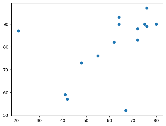
# Plot prestige (y) as a function of income (x).
plt.scatter(x, y)

<matplotlib.collections.PathCollection at 0x7f22897be150>

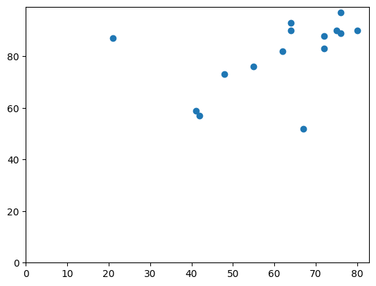
Let’s guess a slope and intercept:

plt.scatter(x, y)
# Put 0, 0 on the plot.
x_min, x_max, y_min, y_max = plt.axis()
limits = [0, x_max, 0, y_max]
plt.axis(limits);

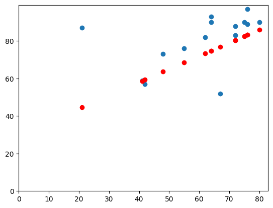
# Our guesses.
b = 0.7
c = 30

# The fitted values
y_hat = b * x + c

plt.scatter(x, y)
plt.plot(x, y_hat, 'ro')
# Put 0, 0 on the plot.
plt.axis(limits);

Remember the notation:

\[ \vec{x} = [x_1, x_2, ... x_n] \]

\[ \vec{y} = [y_1, y_2, ... y_n] \]

The 1D array x is Python’s representation of \(\vec{x}\), and y is \(\vec{y}\).

We calculate our fitted values \(\hat{\vec{y}}\) as

\[ \hat{\vec{y}} = b \vec{x} + c \]

\(b\) and \(c\) are a single values (scalars).

Notice the notation above. The notation assumes that, when we multiply a vector \(\vec{x}\) by a scalar \(b\), that has the effect of multiplying each value in \(\vec{x}\) by the scalar \(b\).

The result of \(b \vec{x}\) is another vector (we’ve called it \(\hat{\vec{y}}\)) that has values \([b x_1, b x_2, ..., b x_n]\).

Not coincidentally, this is also what Numpy understands by mupltiplying the array by the scalar:

bx = b * x
bx

array([43.4, 50.4, 52.5, 38.5, 44.8, 14.7, 44.8, 56. , 46.9, 50.4, 29.4,
       53.2, 53.2, 28.7, 33.6])

The same goes for addition. When we add a scalar \(c\) to a vector, that has the effect of adding the value \(c\) to each value in the vector. So \(b \vec{x} + c\) is \([b x_1 + c, b x_2 + c, ..., b x_n + c]\).

# Adds c to every value of bc
bx + c

array([73.4, 80.4, 82.5, 68.5, 74.8, 44.7, 74.8, 86. , 76.9, 80.4, 59.4,
       83.2, 83.2, 58.7, 63.6])

We find the same parallels between Numpy and mathematical notation for adding and subtracting vectors.

Remember we write the calculation of the errors with:

\[ \vec{e} = \vec{y} - \hat{\vec{y}} \]

That is $\hat{\vec{y}} = [y_1 - \hat{y_1}, y_2 - \hat{y_2}, …, y_n

• \hat{y_n}]$

When we subtract (or add) two vectors, the result is the element by element subtraction of the values in the vectors.

This is Numpy’s idea as well. This means we can write the mathematical formulation more or less directly in code:

# Calculate e vector from y and y_hat
e = y - y_hat
e

array([  8.6,   2.6,   7.5,   7.5,  15.2,  42.3,  18.2,   4. , -24.9,
         7.6,  -2.4,   5.8,  13.8,   0.3,   9.4])

Arrays and lists

You’ve learned that Numpy uses the standard mathematical logic for addition and multiplication of vectors.

You may remember that Python Lists aren’t designed for the same purpose, and they have a different logic for addition and multiplication.

x_as_list = list(x)
x_as_list

[np.int64(62),
 np.int64(72),
 np.int64(75),
 np.int64(55),
 np.int64(64),
 np.int64(21),
 np.int64(64),
 np.int64(80),
 np.int64(67),
 np.int64(72),
 np.int64(42),
 np.int64(76),
 np.int64(76),
 np.int64(41),
 np.int64(48)]

Adding a scalar to a list causes an error:

x_as_list + c

---------------------------------------------------------------------------
TypeError                                 Traceback (most recent call last)
Cell In[14], line 1
----> 1 x_as_list + c

TypeError: can only concatenate list (not "int") to list

Multiplying a list by a scalar p repeats the list \(p\) times:

x_as_list * 3

[np.int64(62),
 np.int64(72),
 np.int64(75),
 np.int64(55),
 np.int64(64),
 np.int64(21),
 np.int64(64),
 np.int64(80),
 np.int64(67),
 np.int64(72),
 np.int64(42),
 np.int64(76),
 np.int64(76),
 np.int64(41),
 np.int64(48),
 np.int64(62),
 np.int64(72),
 np.int64(75),
 np.int64(55),
 np.int64(64),
 np.int64(21),
 np.int64(64),
 np.int64(80),
 np.int64(67),
 np.int64(72),
 np.int64(42),
 np.int64(76),
 np.int64(76),
 np.int64(41),
 np.int64(48),
 np.int64(62),
 np.int64(72),
 np.int64(75),
 np.int64(55),
 np.int64(64),
 np.int64(21),
 np.int64(64),
 np.int64(80),
 np.int64(67),
 np.int64(72),
 np.int64(42),
 np.int64(76),
 np.int64(76),
 np.int64(41),
 np.int64(48)]

Adding two lists concatenates the lists, giving a single list with the elements of the first list followed by the elements of the second:

y_as_list = list(y)
y_as_list

[np.int64(82),
 np.int64(83),
 np.int64(90),
 np.int64(76),
 np.int64(90),
 np.int64(87),
 np.int64(93),
 np.int64(90),
 np.int64(52),
 np.int64(88),
 np.int64(57),
 np.int64(89),
 np.int64(97),
 np.int64(59),
 np.int64(73)]

both = x_as_list + y_as_list
both

[np.int64(62),
 np.int64(72),
 np.int64(75),
 np.int64(55),
 np.int64(64),
 np.int64(21),
 np.int64(64),
 np.int64(80),
 np.int64(67),
 np.int64(72),
 np.int64(42),
 np.int64(76),
 np.int64(76),
 np.int64(41),
 np.int64(48),
 np.int64(82),
 np.int64(83),
 np.int64(90),
 np.int64(76),
 np.int64(90),
 np.int64(87),
 np.int64(93),
 np.int64(90),
 np.int64(52),
 np.int64(88),
 np.int64(57),
 np.int64(89),
 np.int64(97),
 np.int64(59),
 np.int64(73)]

len(both)

30

To repeat then — Numpy makes addition / subtraction and multiplication / division work in the same way on arrays, as we expect from mathematics. See vector space for the gory details.