Dimension reduction with Principal Component Analysis

See the PCA introduction for background.

Start by loading the libraries we need, and doing some configuration:

import numpy as np
import numpy.linalg as npl
# Display array values to 6 digits of precision
np.set_printoptions(precision=6, suppress=True)

import pandas as pd
pd.set_option('mode.copy_on_write', True)

import matplotlib.pyplot as plt

from sklearn.decomposition import PCA
from sklearn.linear_model import LinearRegression
from sklearn.metrics import r2_score

As for the PCA page above, we will use the English Premier League (EPL) table data for this example. See the EPL dataset page for more on this dataset.

df = pd.read_csv('data/premier_league_2021.csv')
df.head()

	rank	team	played	won	drawn	lost	for	against	goal_difference	points	wages_year	keeper	defense	midfield	forward
0	1	Manchester City	38	29	6	3	99	26	73	93	168572	8892	60320	24500	74860
1	2	Liverpool	38	28	8	2	94	26	68	92	148772	14560	46540	47320	40352
2	3	Chelsea	38	21	11	6	76	33	43	74	187340	12480	51220	51100	72540
3	4	Tottenham Hotspur	38	22	5	11	69	40	29	71	110416	6760	29516	30680	43460
4	5	Arsenal	38	22	3	13	61	48	13	69	118074	8400	37024	27300	45350

We want to predict goal difference from spending on the various position types.

We have spending data on keeper defense, midfield and forward.

y = df['goal_difference']
# Divide spending by 10,000 GBP to make numbers easier to read.
X = df[['keeper', 'defense', 'midfield', 'forward']] / 10_000
X.head()

	keeper	defense	midfield	forward
0	0.8892	6.0320	2.450	7.4860
1	1.4560	4.6540	4.732	4.0352
2	1.2480	5.1220	5.110	7.2540
3	0.6760	2.9516	3.068	4.3460
4	0.8400	3.7024	2.730	4.5350

basic_reg = LinearRegression().fit(X, y)
basic_reg.coef_

array([-15.502165,  24.888585,   6.337194,  -5.453179])

How good is the model fit?

fitted = basic_reg.predict(X)
fitted

array([ 58.702936,  48.899144,  48.61422 ,   6.380567,  19.351939,
        15.741829,  -7.189155,  -0.542271, -14.657475, -10.357978,
         5.580663, -11.703874, -33.987123, -10.908234, -38.285969,
        12.001697, -30.212118, -22.902239, -14.680438, -19.84612 ])

full_r2 = r2_score(y, fitted)
full_r2

0.6593261703105764

It turns out the variables (features) are highly correlated, one with another.

X.corr()

	keeper	defense	midfield	forward
keeper	1.000000	0.770622	0.653607	0.836858
defense	0.770622	1.000000	0.792146	0.918498
midfield	0.653607	0.792146	1.000000	0.718424
forward	0.836858	0.918498	0.718424	1.000000

We want to reduce these four variables down to fewer variables, while still capturing the same information.

Let us first run PCA on the four columns:

pca = PCA()
pca = pca.fit(X)

# Scikit-learn's components.
pca.components_

array([[ 0.162258,  0.467464,  0.330791,  0.803571],
       [-0.044097,  0.155829,  0.881052, -0.444433],
       [-0.229876,  0.859756, -0.324967, -0.319959],
       [ 0.958585,  0.134218, -0.093391, -0.233192]])

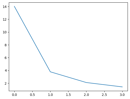
Review the scree-plot of the component weights:

plt.plot(pca.singular_values_)

[<matplotlib.lines.Line2D at 0x7f6b17deb110>]

We can calculate the amount of each row explained by each component, by using fit_transform of the PCA object:

comp_vals = pca.fit_transform(X)
comp_vals

array([[ 4.885102, -0.949893,  1.316577, -0.44375 ],
       [ 2.314803,  2.354588,  0.364081,  0.506204],
       [ 5.211402,  1.339186, -0.33846 , -0.416269],
       [ 1.091745,  0.5195  , -0.478962, -0.387058],
       [ 1.509396,  0.247471,  0.178209, -0.141586],
       [ 8.670343, -1.625328, -0.7396  ,  0.447318],
       [-0.853819, -0.589592,  0.539047,  0.666987],
       [-0.789195,  0.171897,  0.305088,  0.445527],
       [-2.274588, -0.086226,  0.035262, -0.101522],
       [-1.31331 , -0.407973, -0.022812, -0.397283],
       [-1.053835,  0.15501 ,  0.434515, -0.011451],
       [-1.112012,  0.134205, -0.260818, -0.058728],
       [-3.420161, -0.259338, -0.349634, -0.116371],
       [-0.140709, -0.665132, -0.05001 ,  0.032668],
       [-1.937029, -0.105797, -0.84301 ,  0.271394],
       [ 0.893833,  0.785698, -0.225254, -0.144854],
       [-2.666776, -0.942176, -0.100787, -0.215631],
       [-2.68459 , -0.439447,  0.004598, -0.078675],
       [-2.915953,  0.472992, -0.047468, -0.043406],
       [-3.414648, -0.109644,  0.279437,  0.186487]])

If you have followed the PCA introduction page, you will know you can also get these scores by matrix multiplication:

# Getting component values by using matrix multiplication.
demeaned_X = X - np.mean(X, axis=0)
demeaned_X.dot(pca.components_.T)

	0	1	2	3
0	4.885102	-0.949893	1.316577	-0.443750
1	2.314803	2.354588	0.364081	0.506204
2	5.211402	1.339186	-0.338460	-0.416269
3	1.091745	0.519500	-0.478962	-0.387058
4	1.509396	0.247471	0.178209	-0.141586
5	8.670343	-1.625328	-0.739600	0.447318
6	-0.853819	-0.589592	0.539047	0.666987
7	-0.789195	0.171897	0.305088	0.445527
8	-2.274588	-0.086226	0.035262	-0.101522
9	-1.313310	-0.407973	-0.022812	-0.397283
10	-1.053835	0.155010	0.434515	-0.011451
11	-1.112012	0.134205	-0.260818	-0.058728
12	-3.420161	-0.259338	-0.349634	-0.116371
13	-0.140709	-0.665132	-0.050010	0.032668
14	-1.937029	-0.105797	-0.843010	0.271394
15	0.893833	0.785698	-0.225254	-0.144854
16	-2.666776	-0.942176	-0.100787	-0.215631
17	-2.684590	-0.439447	0.004598	-0.078675
18	-2.915953	0.472992	-0.047468	-0.043406
19	-3.414648	-0.109644	0.279437	0.186487

We can use these four columns instead of the original four columns as regressors. Think of the component scores (values) as being a re-expression of the original four columns, that keeps all the same information. When we fit this model, the component scores will get their own coefficients, but because those columns contain the same information as the original columns, the resulting fitted values will be the same as for the original model (within the precision of the calculations).

comp_reg = LinearRegression().fit(comp_vals, y)
comp_fitted = comp_reg.predict(comp_vals)
# The columns and parameters are different, but the fitted values
# are the same.
np.allclose(comp_fitted, fitted)

True

Now we’ve seen the scree-plot, we might conclude that only the first component is important, and we can discard the others. We then just include the first component values a new model.

comp1_vals = comp_vals[:, :1]  # A 2D array with one column
comp1_vals

array([[ 4.885102],
       [ 2.314803],
       [ 5.211402],
       [ 1.091745],
       [ 1.509396],
       [ 8.670343],
       [-0.853819],
       [-0.789195],
       [-2.274588],
       [-1.31331 ],
       [-1.053835],
       [-1.112012],
       [-3.420161],
       [-0.140709],
       [-1.937029],
       [ 0.893833],
       [-2.666776],
       [-2.68459 ],
       [-2.915953],
       [-3.414648]])

comp1_reg = LinearRegression().fit(comp1_vals, y)
comp1_reg.coef_

array([6.833448])

We don’t have quite the same quality of model fit — as measured by \(R^2\), for example, but we have recovered most of the \(R^2\) using this single regressor instead of the original four.

comp1_fitted = comp1_reg.predict(comp1_vals)
r2_score(y, comp1_fitted)

0.42171885321184366

We could improve the fit a little by adding the second component:

comp12_reg = LinearRegression().fit(comp_vals[:, :2], y)
r2_score(y, comp12_reg.predict(comp_vals[:, :2]))

0.525326169266535

And a little more with the third:

comp123_reg = LinearRegression().fit(comp_vals[:, :3], y)
r2_score(y, comp123_reg.predict(comp_vals[:, :3]))

0.6484639642971903

Until we get the full \(R^2\) with all four components (which gives the same underling model as using the original four regressors):

comp_reg = LinearRegression().fit(comp_vals, y)
r2_score(y, comp_reg.predict(comp_vals))

0.6593261703105762