Attack or defense? An example of multiple regression

What should you pay for, if you want to win the English Premier League?

import numpy as np
import pandas as pd
pd.set_option('mode.copy_on_write', True)
import matplotlib.pyplot as plt

# Show arrays without exponential notation, 6 digits of precision.
np.set_printoptions(suppress=True, precision=6)

<Token var=<ContextVar name='format_options' default={'edgeitems': 3, 'threshold': 1000, 'floatmode': 'maxprec', 'precision': 8, 'suppress': False, 'linewidth': 75, 'nanstr': 'nan', 'infstr': 'inf', 'sign': '-', 'formatter': None, 'legacy': 9223372036854775807, 'override_repr': None} at 0x7fa3d06db330> at 0x7fa3d6585d40>

# For minimize.
import scipy.optimize as spo
# For linregress
import scipy.stats as sps
# For running statistical models.
import statsmodels.formula.api as smf

We load the data on wage spends in the 2021-2022 English Premier League (EPL).

See the EPL dataset page for more details.

df = pd.read_csv('data/premier_league_2021.csv')
df.head()

	rank	team	played	won	drawn	lost	for	against	goal_difference	points	wages_year	keeper	defense	midfield	forward
0	1	Manchester City	38	29	6	3	99	26	73	93	168572	8892	60320	24500	74860
1	2	Liverpool	38	28	8	2	94	26	68	92	148772	14560	46540	47320	40352
2	3	Chelsea	38	21	11	6	76	33	43	74	187340	12480	51220	51100	72540
3	4	Tottenham Hotspur	38	22	5	11	69	40	29	71	110416	6760	29516	30680	43460
4	5	Arsenal	38	22	3	13	61	48	13	69	118074	8400	37024	27300	45350

Notice that we have the total yearly wage bill for each team, as well as the individual spends on the keeper, defense, midfield and forwards.

There are 20 EPL teams.

len(df)

20

The data frame describe method gives useful statistics for all the numerical columns.

df.describe()

	rank	played	won	drawn	lost	for	against	goal_difference	points	wages_year	keeper	defense	midfield	forward
count	20.00000	20.0	20.000000	20.0000	20.000000	20.000000	20.000000	20.000000	20.00000	20.000000	20.000000	20.000000	20.000000	20.00000
mean	10.50000	38.0	14.600000	8.8000	14.600000	53.550000	53.550000	0.000000	52.60000	91201.650000	7826.900000	28240.350000	20573.600000	34560.80000
std	5.91608	0.0	6.762124	3.5333	6.451438	19.454332	16.223683	33.829293	19.34561	56966.366691	6188.993744	15652.908004	13186.983145	26175.61029
min	1.00000	38.0	5.000000	3.0000	2.000000	23.000000	26.000000	-61.000000	22.00000	28606.000000	2080.000000	8686.000000	3980.000000	6280.00000
25%	5.75000	38.0	10.500000	6.0000	11.750000	42.000000	43.750000	-20.000000	39.75000	47872.500000	3065.000000	14925.000000	11747.500000	17805.50000
50%	10.50000	38.0	13.000000	8.0000	14.500000	49.000000	53.500000	-2.000000	50.00000	75622.000000	7410.000000	26718.000000	16386.000000	26410.00000
75%	15.25000	38.0	17.250000	11.0000	18.000000	61.250000	63.000000	10.000000	60.75000	112330.500000	9462.500000	32890.000000	28145.000000	41129.00000
max	20.00000	38.0	29.000000	15.0000	27.000000	99.000000	84.000000	73.000000	93.00000	238780.000000	28600.000000	60480.000000	51100.000000	112780.00000

Notice mean (and sum) goal_difference is 0. This must be so, because every goal counts 1 positive for the scoring team, and 1 negative for the other team.

The shape attribute of the data frame gives the number of rows and the number of columns.

df.shape

(20, 15)

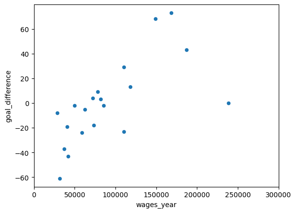
We are interested in whether the wage spend can predict the goal difference. Maybe if you pay more, you score more goals and keep more goals out.

df.plot.scatter(x='wages_year', y='goal_difference')
# We show the y-axis so we can estimate the intercept.
plt.xlim(0, 300000)

(0.0, 300000.0)

We want a best-fit line to these data.

We can use a cost-function to tell use the quality of the line. Low cost corresponds to a good line.

We use the usual sum-of-squared errors as the cost.

def sse_cost(params, x, y):
    """ Sum of squared error cost function
    """
    b, c = params
    y_hat = b * x + c
    errors = y - y_hat
    return np.sum(errors ** 2)

Here are some estimates for the intercept and slope, by eye-balling the graph.

guessed_intercept = -40
# Goal difference increases by about 20 for a £50,000 increase in spend.
# Slope is rise (in y) divided by run (over x).
guessed_slope = 20 / 50000
guessed_slope

0.0004

We use minimize and the 'powell' method to find the values for slope and intercept (params) that give the lowest values for the cost function.

res = spo.minimize(sse_cost, [guessed_intercept, guessed_slope],
                   method='powell',
                   args=(df['wages_year'], df['goal_difference']))
res

 message: Optimization terminated successfully.
 success: True
  status: 0
     fun: 12070.170784478678
       x: [ 3.728e-04 -3.360e+01]
     nit: 34
   direc: [[ 5.352e-07  1.264e-01]
           [ 8.769e-07  8.421e-02]]
    nfev: 833

These are the parameters (the slope and the intercept):

res.x

array([  0.000373, -33.601334])

If we run linregress, this uses the mathematics of sum-of-squares to get the minimizing slope and intercept.

lr_res = sps.linregress(df['wages_year'], df['goal_difference'])
lr_res

LinregressResult(slope=np.float64(0.00039689691255513594), intercept=np.float64(-36.197653304934114), rvalue=np.float64(0.6683490305377195), pvalue=np.float64(0.0012767215478024995), stderr=np.float64(0.0001041171418862387), intercept_stderr=np.float64(11.11698541165042))

We suspect that minimize was less accurate than sps.linregress; the very small slope may mean that minimize gives up searching for the exact correct slope when it has got very close.

Here’s the cost function value from the parameters from minimize.

sse_cost(res.x, df['wages_year'], df['goal_difference'])

np.float64(12070.170784478678)

The parameters from sps.linregress are slightly better — they give a somewhat lower value for the cost function.

sse_cost([lr_res.slope, lr_res.intercept], df['wages_year'], df['goal_difference'])

np.float64(12031.163363559293)

In data science practice, we often use these least-squares cost functions, and we can use convenient libraries for these calculations. statsmodels is a useful library for these general models.

Using statsmodels, we first create a model, that encodes the relationship we’re investigating, along with the data.

sm_model = smf.ols('goal_difference ~ wages_year', data=df)
sm_model

<statsmodels.regression.linear_model.OLS at 0x7fa39854b710>

Once we have specified this model, we can use the .fit method of the new model to calculate the least-squares parameters.

sm_fit = sm_model.fit()
sm_fit

<statsmodels.regression.linear_model.RegressionResultsWrapper at 0x7fa37f780b90>

Finally, we can use the .summary method of the fit result, to show a detailed display of the parameters and other calculations from the fit.

sm_fit.summary()

OLS Regression Results

Dep. Variable:	goal_difference	R-squared:	0.447
Model:	OLS	Adj. R-squared:	0.416
Method:	Least Squares	F-statistic:	14.53
Date:	Tue, 03 Sep 2024	Prob (F-statistic):	0.00128
Time:	10:05:32	Log-Likelihood:	-92.374
No. Observations:	20	AIC:	188.7
Df Residuals:	18	BIC:	190.7
Df Model:	1
Covariance Type:	nonrobust

	coef	std err	t	P>|t|	[0.025	0.975]
Intercept	-36.1977	11.117	-3.256	0.004	-59.554	-12.842
wages_year	0.0004	0.000	3.812	0.001	0.000	0.001

Omnibus:	1.288	Durbin-Watson:	1.194
Prob(Omnibus):	0.525	Jarque-Bera (JB):	0.487
Skew:	-0.375	Prob(JB):	0.784
Kurtosis:	3.142	Cond. No.	2.05e+05

Notes:
[1] Standard Errors assume that the covariance matrix of the errors is correctly specified.
[2] The condition number is large, 2.05e+05. This might indicate that there are
strong multicollinearity or other numerical problems.

Defense or attack?

Here’s a reminder of the columns of data we have.

df.head()

	rank	team	played	won	drawn	lost	for	against	goal_difference	points	wages_year	keeper	defense	midfield	forward
0	1	Manchester City	38	29	6	3	99	26	73	93	168572	8892	60320	24500	74860
1	2	Liverpool	38	28	8	2	94	26	68	92	148772	14560	46540	47320	40352
2	3	Chelsea	38	21	11	6	76	33	43	74	187340	12480	51220	51100	72540
3	4	Tottenham Hotspur	38	22	5	11	69	40	29	71	110416	6760	29516	30680	43460
4	5	Arsenal	38	22	3	13	61	48	13	69	118074	8400	37024	27300	45350

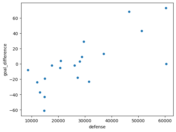
Our question now is — should we spend on defense, or spend on attack (forwards)?

Here’s the plot of defense spending as a function of goal difference.

df.plot.scatter(x='defense', y='goal_difference')

<Axes: xlabel='defense', ylabel='goal_difference'>

And the relationship of forward spending and goal difference.

df.plot.scatter(x='forward', y='goal_difference')

<Axes: xlabel='forward', ylabel='goal_difference'>

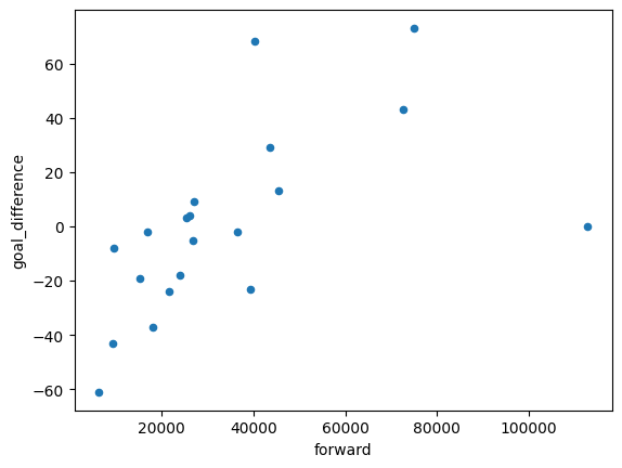
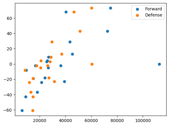
Notice that both, on their own, have strongly positive relationships.

Here we put both on the same plot.

plt.scatter(df['forward'], df['goal_difference'], label='Forward')
plt.scatter(df['defense'], df['goal_difference'], label='Defense')
plt.legend()

<matplotlib.legend.Legend at 0x7fa37d6432d0>

Here we calculate the simple regression models for each. Notice the chained execution for calculating the model, then the fit, and then the summary.

smf.ols('goal_difference ~ defense', data=df).fit().summary()

OLS Regression Results

Dep. Variable:	goal_difference	R-squared:	0.549
Model:	OLS	Adj. R-squared:	0.524
Method:	Least Squares	F-statistic:	21.94
Date:	Tue, 03 Sep 2024	Prob (F-statistic):	0.000185
Time:	10:05:32	Log-Likelihood:	-90.322
No. Observations:	20	AIC:	184.6
Df Residuals:	18	BIC:	186.6
Df Model:	1
Covariance Type:	nonrobust

	coef	std err	t	P>|t|	[0.025	0.975]
Intercept	-45.2366	10.976	-4.121	0.001	-68.297	-22.176
defense	0.0016	0.000	4.684	0.000	0.001	0.002

Omnibus:	1.906	Durbin-Watson:	1.356
Prob(Omnibus):	0.386	Jarque-Bera (JB):	1.197
Skew:	-0.597	Prob(JB):	0.550
Kurtosis:	2.891	Cond. No.	6.75e+04

Notes:
[1] Standard Errors assume that the covariance matrix of the errors is correctly specified.
[2] The condition number is large, 6.75e+04. This might indicate that there are
strong multicollinearity or other numerical problems.

smf.ols('goal_difference ~ forward', data=df).fit().summary()

OLS Regression Results

Dep. Variable:	goal_difference	R-squared:	0.332
Model:	OLS	Adj. R-squared:	0.295
Method:	Least Squares	F-statistic:	8.934
Date:	Tue, 03 Sep 2024	Prob (F-statistic):	0.00787
Time:	10:05:32	Log-Likelihood:	-94.262
No. Observations:	20	AIC:	192.5
Df Residuals:	18	BIC:	194.5
Df Model:	1
Covariance Type:	nonrobust

	coef	std err	t	P>|t|	[0.025	0.975]
Intercept	-25.7248	10.698	-2.405	0.027	-48.200	-3.250
forward	0.0007	0.000	2.989	0.008	0.000	0.001

Omnibus:	1.089	Durbin-Watson:	1.010
Prob(Omnibus):	0.580	Jarque-Bera (JB):	0.161
Skew:	0.120	Prob(JB):	0.923
Kurtosis:	3.369	Cond. No.	7.23e+04

Notes:
[1] Standard Errors assume that the covariance matrix of the errors is correctly specified.
[2] The condition number is large, 7.23e+04. This might indicate that there are
strong multicollinearity or other numerical problems.

Now we are interesting in taking both defense and forward spending into account at the same time.

This is multiple regression.

Notice that in multiple regression, we calculate the fitted \(\hat{\vec{y}}\) values by adding to together the components due to the first predictor, and that due to the second predictor, and the intercept.

def sse_multi(params, X, y):
    """ Multiple regression sum of squared error

    Parameters
    ----------
    params : slopes and intercept
    X : array
        2D array of predictor columns.
    y : array
        1D array of outcome vector.

    Returns
    -------
    cfv : float
        Cost function value
    """
    n, p = X.shape
    y_hat = np.zeros(n)
    for col_no in range(p):  # Go through each column.
        col = X[:, col_no]  # Get the relevant column from X
        fit_for_this_col = col * params[col_no]  # Multiply by corresponding parameter
        y_hat = y_hat + fit_for_this_col
    y_hat = y_hat + params[-1]  # Add the intercept
    errors = y - y_hat
    return np.sum(errors ** 2)

We compile the 2D array containing the two predictor columns, by taking two columns out of the data frame, and converting to an array.

X = np.array(df[['defense', 'forward']])
X

array([[ 60320,  74860],
       [ 46540,  40352],
       [ 51220,  72540],
       [ 29516,  43460],
       [ 37024,  45350],
       [ 60480, 112780],
       [ 28860,  27040],
       [ 28040,  25440],
       [ 17640,  16790],
       [ 20736,  26820],
       [ 27276,  24040],
       [ 20930,  26000],
       [  8686,   9620],
       [ 26160,  36470],
       [ 12137,  21530],
       [ 31512,  39310],
       [ 13150,  18144],
       [ 14940,  15110],
       [ 14880,   9280],
       [ 14760,   6280]])

Next we use minimize to find the three parameters that minimize the cost function. We found that both powell and the default methods gave warnings about failing to reach good results, so we tried the nelder-mead method.

min_res_2 = spo.minimize(sse_multi, [0.001, 0.001, -36],
                         method='nelder-mead',
                         args=(X, df['goal_difference']))
min_res_2

       message: Optimization terminated successfully.
       success: True
        status: 0
           fun: 8270.703854709001
             x: [ 2.933e-03 -8.665e-04 -5.288e+01]
           nit: 107
          nfev: 192
 final_simplex: (array([[ 2.933e-03, -8.665e-04, -5.288e+01],
                       [ 2.933e-03, -8.665e-04, -5.288e+01],
                       [ 2.933e-03, -8.665e-04, -5.288e+01],
                       [ 2.933e-03, -8.665e-04, -5.288e+01]]), array([ 8.271e+03,  8.271e+03,  8.271e+03,  8.271e+03]))

Here are the parameters:

• slope for defense

• slope for attack

• intercept.

min_res_2.x

array([  0.002933,  -0.000867, -52.875186])

We can do the same parameter estimating using statsmodels in our case, because we are using the standard least-squares cost function.

fitted = smf.ols('goal_difference ~ defense + forward', data=df).fit()
fitted.summary()

OLS Regression Results

Dep. Variable:	goal_difference	R-squared:	0.620
Model:	OLS	Adj. R-squared:	0.575
Method:	Least Squares	F-statistic:	13.85
Date:	Tue, 03 Sep 2024	Prob (F-statistic):	0.000270
Time:	10:05:32	Log-Likelihood:	-88.626
No. Observations:	20	AIC:	183.3
Df Residuals:	17	BIC:	186.2
Df Model:	2
Covariance Type:	nonrobust

	coef	std err	t	P>|t|	[0.025	0.975]
Intercept	-52.8752	11.236	-4.706	0.000	-76.581	-29.169
defense	0.0029	0.001	3.587	0.002	0.001	0.005
forward	-0.0009	0.000	-1.772	0.094	-0.002	0.000

Omnibus:	1.441	Durbin-Watson:	1.303
Prob(Omnibus):	0.486	Jarque-Bera (JB):	1.207
Skew:	-0.548	Prob(JB):	0.547
Kurtosis:	2.501	Cond. No.	1.21e+05

Notes:
[1] Standard Errors assume that the covariance matrix of the errors is correctly specified.
[2] The condition number is large, 1.21e+05. This might indicate that there are
strong multicollinearity or other numerical problems.

The found parameters are almost exactly what we found with minimize.

fitted.params

Intercept   -52.875175
defense       0.002933
forward      -0.000867
dtype: float64

The parameters make us think that we gain very little — or even lose — by extra spending on forwards, given a particular level of spending on defense.

Another way of looking at this is to first remove (“regress out”) the effect of spending on defense, leaving the errors (AKA residuals). The residuals are what remains of goal difference after we have done the best job we can (in the least-squares sense) of removing the effect of spending on defense.

defense_only_fit = smf.ols('goal_difference ~ defense', data=df).fit()
defense_only_fit.params

Intercept   -45.236577
defense       0.001602
dtype: float64

Here we calculate residuals (errors) left over after using the fit from the defense-only model.

y_hat = defense_only_fit.params['defense'] * df['defense'] + defense_only_fit.params['Intercept']
errors = df['goal_difference'] - y_hat
errors

0     21.613471
1     38.686853
2      6.190233
3     26.956610
4     -1.070019
5    -51.642824
6      8.007419
7      3.320929
8     14.980085
9      7.020783
10   -16.455264
11    15.710025
12    23.322978
13     1.332392
14     1.795021
15   -28.240666
16   -12.827644
17     2.305058
18   -21.598831
19   -39.406610
dtype: float64

In fact Statsmodels is kind enough to calculate these for us, by default, in the resid attribute of the fit.

defense_only_fit.resid

0     21.613471
1     38.686853
2      6.190233
3     26.956610
4     -1.070019
5    -51.642824
6      8.007419
7      3.320929
8     14.980085
9      7.020783
10   -16.455264
11    15.710025
12    23.322978
13     1.332392
14     1.795021
15   -28.240666
16   -12.827644
17     2.305058
18   -21.598831
19   -39.406610
dtype: float64

We can take the residual — left over — values, and put them back into the data frame, so Statmodels can do another fit.

df['without_defense'] = fitted.resid
df

	rank	team	played	won	drawn	lost	for	against	goal_difference	points	wages_year	keeper	defense	midfield	forward	without_defense
0	1	Manchester City	38	29	6	3	99	26	73	93	168572	8892	60320	24500	74860	13.837431
1	2	Liverpool	38	28	8	2	94	26	68	92	148772	14560	46540	47320	40352	19.349313
2	3	Chelsea	38	21	11	6	76	33	43	74	187340	12480	51220	51100	72540	8.515417
3	4	Tottenham Hotspur	38	22	5	11	69	40	29	71	110416	6760	29516	30680	43460	32.970125
4	5	Arsenal	38	22	3	13	61	48	13	69	118074	8400	37024	27300	45350	-3.411476
5	6	Manchester United	38	16	10	12	57	57	0	58	238780	28600	60480	36920	112780	-26.773404
6	7	West Ham United	38	16	8	14	60	51	9	56	77936	11856	28860	10180	27040	0.665784
7	8	Leicester City	38	14	10	14	62	59	3	52	81590	10040	28040	18070	25440	-4.315766
8	9	Brighton and Hove Albion	38	12	15	11	42	44	-2	51	49820	3120	17640	12270	16790	13.689769
9	10	Wolverhampton Wanderers	38	15	6	17	38	43	-5	51	62756	2120	20736	13080	26820	10.301066
10	11	Newcastle United	38	13	10	15	44	62	-18	49	73308	4940	27276	17052	24040	-24.288248
11	12	Crystal Palace	38	11	15	12	50	46	4	48	71910	6000	20930	18980	26000	18.021561
12	13	Brentford	38	13	7	18	48	56	-8	46	28606	2080	8686	8220	9620	27.736951
13	14	Aston Villa	38	13	6	19	52	54	-2	45	85330	8320	26160	14380	36470	5.755570
14	15	Southampton	38	9	13	16	43	67	-24	40	58657	9270	12137	15720	21530	11.936166
15	16	Everton	38	11	6	21	43	66	-23	39	110202	8060	31512	31320	39310	-28.479761
16	17	Leeds United	38	9	11	18	42	79	-37	38	37354	2080	13150	3980	18144	-6.968775
17	18	Burnley	38	7	14	17	34	53	-19	35	40830	2900	14940	7880	15110	3.152527
18	19	Watford	38	6	5	27	34	77	-43	23	42030	2580	14880	15290	9280	-25.723314
19	20	Norwich City	38	5	7	26	23	84	-61	22	31750	3480	14760	7230	6280	-45.970937

Now we look to see if the forward spending can predict what is left over, after taking into account the effect of defense spending on goal difference:

smf.ols('without_defense ~ forward', data=df).fit().summary()

OLS Regression Results

Dep. Variable:	without_defense	R-squared:	0.000
Model:	OLS	Adj. R-squared:	-0.056
Method:	Least Squares	F-statistic:	0.000
Date:	Tue, 03 Sep 2024	Prob (F-statistic):	1.00
Time:	10:05:32	Log-Likelihood:	-88.626
No. Observations:	20	AIC:	181.3
Df Residuals:	18	BIC:	183.2
Df Model:	1
Covariance Type:	nonrobust

	coef	std err	t	P>|t|	[0.025	0.975]
Intercept	-1.288e-14	8.071	-1.6e-15	1.000	-16.956	16.956
forward	-1.335e-18	0.000	-7.11e-15	1.000	-0.000	0.000

Omnibus:	1.441	Durbin-Watson:	1.303
Prob(Omnibus):	0.486	Jarque-Bera (JB):	1.207
Skew:	-0.548	Prob(JB):	0.547
Kurtosis:	2.501	Cond. No.	7.23e+04

Notes:
[1] Standard Errors assume that the covariance matrix of the errors is correctly specified.
[2] The condition number is large, 7.23e+04. This might indicate that there are
strong multicollinearity or other numerical problems.

It appears that this two-stage procedure gives a similar result to the one we saw before — once we have accounted for spending on defense, spending on forwards is no longer important, in these models.