2D arrays, images, optimization

Here we use a 2D array to look at the search for the best (least-squares) line for a simple regression.

import numpy as np
import pandas as pd
pd.set_option('mode.copy_on_write', True)
import matplotlib.pyplot as plt

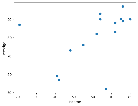
We return again to the income and prestige data from Duncan [Dun61].

df = pd.read_csv('data/Duncan_Occupational_Prestige.csv')
# Select the first 15 rows (occupations).
top_15 = df.head(15)
top_15

	name	type	income	education	prestige
0	accountant	prof	62	86	82
1	pilot	prof	72	76	83
2	architect	prof	75	92	90
3	author	prof	55	90	76
4	chemist	prof	64	86	90
5	minister	prof	21	84	87
6	professor	prof	64	93	93
7	dentist	prof	80	100	90
8	reporter	wc	67	87	52
9	engineer	prof	72	86	88
10	undertaker	prof	42	74	57
11	lawyer	prof	76	98	89
12	physician	prof	76	97	97
13	welfare.worker	prof	41	84	59
14	teacher	prof	48	91	73

We will be doing a regression predicting 'prestige' as a function of 'income'.

x = top_15['income']
y = top_15['prestige']

Plot these observations.

plt.scatter(x, y)
plt.xlabel('Income')
plt.ylabel('Prestige')

Text(0, 0.5, 'Prestige')

Start with a guess for the slope and intercept of a line to predict the y ('prestige') values from the x ('income') values.

b = 0.7  # Guessed slope.
c = 30  # Guessed intercept.

To find the best least-squares slope, we first need a function to calculate the Root Mean Squared Error (RMSE) for a given slope and intercept, and given x and y vectors.

We’ve chosen RMSE as the cost (or loss) function here, but we could equally have chosen the sum of squared errors (SSE) or the mean squared error (MSE); these measures go up and down together, so when we have found the slope and intercept minimizing the RMSE, that same slope and intercept will minimize SSE and MSE.

def rmse_for_b_and_c(b, c, x, y):
    """ Root mean squared error for slope `b` intercept `c`
    """
    y_hat = b * x + c
    e = y - y_hat
    e2 = e ** 2
    return np.sqrt(np.mean(e2))

We calculate the RMSE for our guessed slope and intercept:

rmse_for_b_and_c(b, c, x, y)

np.float64(15.398809477791893)

Just to make sure, we calculated the RMSE again, outside the function, to make sure we’re returning the correct result:

y_hat = b * x + c
e = y - y_hat
np.sqrt(np.mean(e ** 2))

np.float64(15.398809477791893)

We are now going to do a brute-force search for the best RMSE slope an intercept.

A brute-force search is where we search a wide range of slope and intercept pairs and select the pair that gives the lowest RMSE.

Alternative methods are using scipy.optimize.minimize to select sensible slopes and intercepts to try for us, or to use the mathematical short-cuts of routines like scipy.statistics.linregress. These last will work for our case — looking for the slope, intercept minimizing the squared error (or RMSE in our case), but we can’t use them for other calculations of the error.

First we select some slopes to try, based on looking at the scatterplot above.

# Make 250 slopes by taking equally spaced values starting at 0
# and ending at 0.5.
candidate_slopes = np.linspace(0, 0.5, 250)
candidate_slopes[:10]

array([0.        , 0.00200803, 0.00401606, 0.0060241 , 0.00803213,
       0.01004016, 0.01204819, 0.01405622, 0.01606426, 0.01807229])

# Make 250 intercepts by taking equally spaced values starting at 40
# and ending at 70.
candidate_inters = np.linspace(40, 70, 250)
candidate_inters[:10]

array([40.        , 40.12048193, 40.24096386, 40.36144578, 40.48192771,
       40.60240964, 40.72289157, 40.84337349, 40.96385542, 41.08433735])

These are the number of candidate slopes and intercepts. In our case, the np.linspace calls above dictate these numbers will be 250.

n_slopes = len(candidate_slopes)
n_inters = len(candidate_inters)

Make a two-dimensional array to store the RMSE values corresponding to each slope / intercept pair.

rmses = np.zeros([n_slopes, n_inters])
rmses.shape

(250, 250)

We are next going to start using Python’s range to make sequences of integer values in our for loops.

Up until now, we have been using Numpys arange to make sequential arrays of numbers, and feeding these into our for loops:

np.arange(1, 11)

array([ 1,  2,  3,  4,  5,  6,  7,  8,  9, 10])

# The old way
for i in np.arange(1, 11):
    print(i)

1
2
3
4
5
6
7
8
9
10

Now we are going to switch to the more common Python idiom of using range in our for loops, instead of np.arange. range takes the same arguments as does np.arange — start, stop and step — but returns a range object.

my_r = range(1, 11)
my_r

range(1, 11)

type(my_r)

range

len(my_r)

10

my_r here is an object that refers to the sequence of numbers 1, 2, … 10 — but does not directly contain this sequence.

We can force the range object to create and return the corresponding numbers using e.g. list. list asks the range object for it’s sequence, and range returns them one by one, from which list compiles the list.

list(my_r)

[1, 2, 3, 4, 5, 6, 7, 8, 9, 10]

We will use range in place of np.arange as the right-hand-side of for loops — providing the sequence from which we will fill the loop variable. In the next cell, the loop variable is v:

for v in range(5):
    print(v)

0
1
2
3
4

Back to the problem. We loop through each slope in turn. For each slope value we loop through each intercept value in turn. For the given slope and intercept, we calculate the RMSE value, and store it in corresponding location in the rmses array, where the row position comes from the position of the slope value, and the column position comes from the position of the intercept value.

for slope_no in range(n_slopes):
    b = candidate_slopes[slope_no]  # Get the corresponding slope.
    for inter_no in range(n_inters):
        c = candidate_inters[inter_no]  # Get the corresponding intercept.
        rmse = rmse_for_b_and_c(b, c, x, y)  # Calculate RMSE.
        rmses[slope_no, inter_no] = rmse  # Store in rmses array.

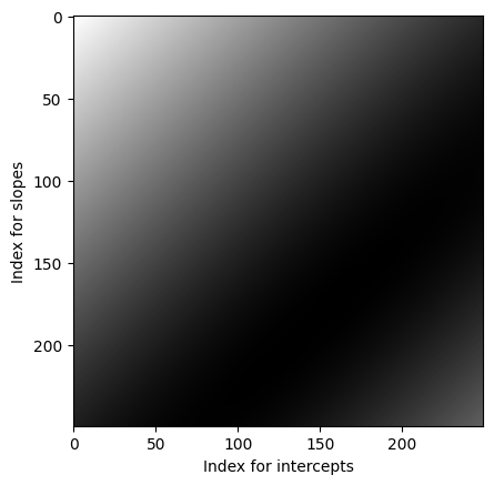
If we plt.imshow the rmses array, we see a dark valley corresponding to low values of RMSE for the corresponding slope, intercept pairs. Bright areas are for much higher RMSEs.

plt.imshow(rmses, cmap='gray')
plt.ylabel('Index for slopes')
plt.xlabel('Index for intercepts')

Text(0.5, 0, 'Index for intercepts')

Next we want to find the slope and intercept corresponding to the minimum RMSE value we found in the rmses array.

To do this, we are going to need np.where. It can tell us the location of values in terms of index position.

Consider a one-dimensional array like this:

an_arr = np.array([1, 32, 99, 4, 2])
an_arr

array([ 1, 32, 99,  4,  2])

We can make a Boolean array with True where the values are equal to 99, and False otherwise:

an_arr == 99

array([False, False,  True, False, False])

np.where calculates where the True value(s) are, in terms of index position. In our case, the 99 value is at position (index) 3 in the array:

np.where(an_arr == 99)

(array([2]),)

We can apply the same logic to two-dimensions.

First we find the minimum RMSE value over the whole array:

min_rmse = np.min(rmses)
min_rmse

np.float64(12.24410485663457)

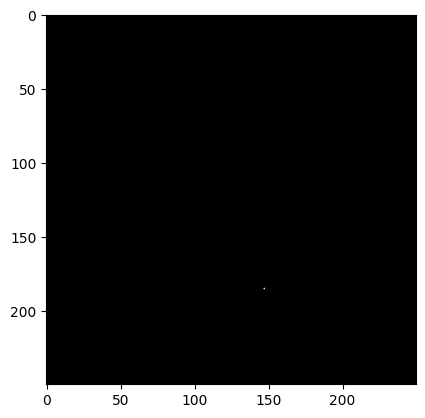
Next we calculate a 2D Boolean array, of the same shape as rmses, but having True in the element corresponding the minimum value, and False otherwise.

is_min = rmses == min_rmse
is_min[:10, :10]

array([[False, False, False, False, False, False, False, False, False,
        False],
       [False, False, False, False, False, False, False, False, False,
        False],
       [False, False, False, False, False, False, False, False, False,
        False],
       [False, False, False, False, False, False, False, False, False,
        False],
       [False, False, False, False, False, False, False, False, False,
        False],
       [False, False, False, False, False, False, False, False, False,
        False],
       [False, False, False, False, False, False, False, False, False,
        False],
       [False, False, False, False, False, False, False, False, False,
        False],
       [False, False, False, False, False, False, False, False, False,
        False],
       [False, False, False, False, False, False, False, False, False,
        False]])

Again, plt.imshow will show us the single True value as a white dot. All the other values in this array are black (False).

plt.imshow(is_min, cmap='gray', interpolation=None)

<matplotlib.image.AxesImage at 0x7f5f5fcf2050>

Back to np.where. If we call this on the is_min 2D Boolean array, it returns the row and column indices of the single True value in the array. Notice the use of unpacking to unpack the two returned arrays (row coordinates and column coordinates).

min_row, min_col = np.where(is_min)
min_row, min_col

(array([185]), array([147]))

Now we know the row position of the minimum, we can work back to the corresponding slope value:

best_slope = candidate_slopes[min_row]
best_slope

array([0.37148594])

Similarly, for the corresponding intercept value:

best_inter = candidate_inters[min_col]
best_inter

array([57.71084337])

Let’s run the mathematical calculation to find the best slope and intercept.

import scipy.stats as sps

res = sps.linregress(x, y)
res

LinregressResult(slope=np.float64(0.37105943152454773), intercept=np.float64(57.7653746770026), rvalue=np.float64(0.4376748771939141), pvalue=np.float64(0.10276532267999378), stderr=np.float64(0.21141912223374978), intercept_stderr=np.float64(13.336173440465936))

Notice that the mathematical (Scipy) calculation differs slightly from our brute-force search values. This is because our brute-force search didn’t try every possible slope and intercept value, only the values we got from our np.linspace calls above.

As we’d expect though, the RMSE from the Scipy’s high-precision estimate is a tiny-bit lower than our low-precision np.linspace estimate:

rmse_for_b_and_c(best_slope, best_inter, x, y)

np.float64(12.24410485663457)

rmse_for_b_and_c(res.slope, res.intercept, x, y)

np.float64(12.244069738260368)

References

Dun61

Otis Dudley Duncan. A socioeconomic index for all occupations. In Albert J Reiss, Otis Dudley Duncan, Paul K Hatt, and Douglass Cecil North, editors, Occupations and social status, pages 109–161. Free Press, New York, 1961.