Naive Bayes classifiers

import numpy as np
import pandas as pd
import matplotlib.pyplot as plt
pd.set_option('mode.copy_on_write', True)

Also see: Naive Bayes classifiers in the Python Data Science Handbook.

import seaborn as sns

penguins = pd.read_csv('data/penguins.csv').dropna()
penguins

	species	island	bill_length_mm	bill_depth_mm	flipper_length_mm	body_mass_g	sex	year
0	Adelie	Torgersen	39.1	18.7	181.0	3750.0	male	2007
1	Adelie	Torgersen	39.5	17.4	186.0	3800.0	female	2007
2	Adelie	Torgersen	40.3	18.0	195.0	3250.0	female	2007
4	Adelie	Torgersen	36.7	19.3	193.0	3450.0	female	2007
5	Adelie	Torgersen	39.3	20.6	190.0	3650.0	male	2007
...	...	...	...	...	...	...	...	...
339	Chinstrap	Dream	55.8	19.8	207.0	4000.0	male	2009
340	Chinstrap	Dream	43.5	18.1	202.0	3400.0	female	2009
341	Chinstrap	Dream	49.6	18.2	193.0	3775.0	male	2009
342	Chinstrap	Dream	50.8	19.0	210.0	4100.0	male	2009
343	Chinstrap	Dream	50.2	18.7	198.0	3775.0	female	2009

333 rows × 8 columns

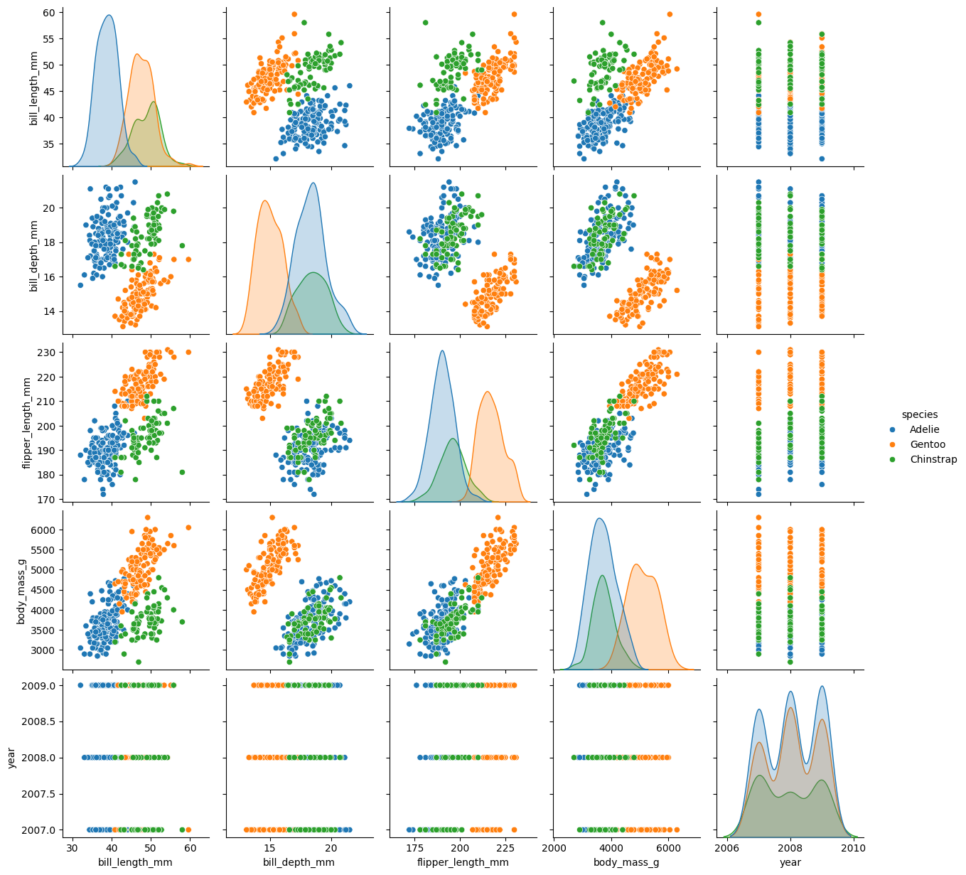
sns.pairplot(penguins, hue="species")

<seaborn.axisgrid.PairGrid at 0x7f5ef1664910>

species_names = ['Chinstrap', 'Gentoo']

df = penguins.loc[
    penguins['species'].isin(species_names),
    ['species', 'body_mass_g', 'bill_depth_mm']
]
df

	species	body_mass_g	bill_depth_mm
152	Gentoo	4500.0	13.2
153	Gentoo	5700.0	16.3
154	Gentoo	4450.0	14.1
155	Gentoo	5700.0	15.2
156	Gentoo	5400.0	14.5
...	...	...	...
339	Chinstrap	4000.0	19.8
340	Chinstrap	3400.0	18.1
341	Chinstrap	3775.0	18.2
342	Chinstrap	4100.0	19.0
343	Chinstrap	3775.0	18.7

187 rows × 3 columns

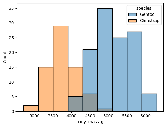
sns.histplot(data=df, x="body_mass_g", hue="species")

<Axes: xlabel='body_mass_g', ylabel='Count'>

by_species = df.groupby('species')
bm_by_species = by_species['body_mass_g']

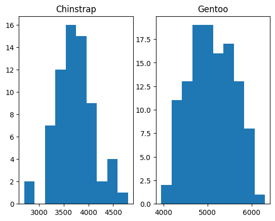
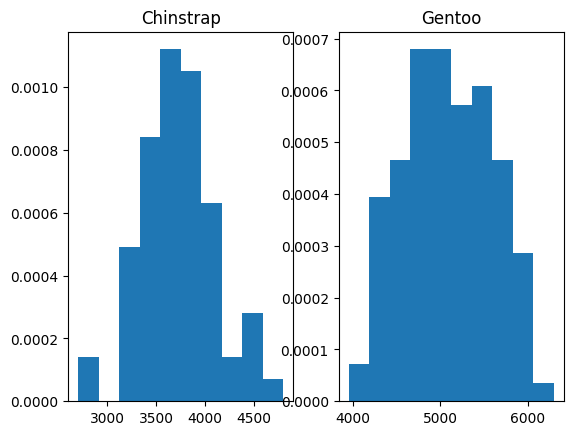
fig, axes = plt.subplots(1, 2)
axes[0].hist(bm_by_species.get_group('Chinstrap'))
axes[0].set_title('Chinstrap')
axes[1].hist(bm_by_species.get_group('Gentoo'));
axes[1].set_title('Gentoo')

Text(0.5, 1.0, 'Gentoo')

Enumerate

While we are here — we introduce enumerate.

Imagine we need both the elements in a list, and the position of that element:

position_no = 0  # A variable to keep track of the position (index).
for name in species_names:
    print('Group', position_no, 'name is', name)
    position_no = position_no + 1  # We have to increment the position.

Group 0 name is Chinstrap
Group 1 name is Gentoo

We can avoid the extra variable by using enumerate, wrapped around the set of things we want to process. enumerate returns two things at each step — the position (index), and the next element from the set of things.

for position_no, name in enumerate(species_names):
    print('Group', position_no, 'name is', name)

Group 0 name is Chinstrap
Group 1 name is Gentoo

We use enumerate to do the plots more neatly below.

The plots again:

fig, axes = plt.subplots(1, 2)
for i, name in enumerate(species_names):
    axes[i].hist(bm_by_species.get_group(name))
    axes[i].set_title(name)

Towards classification with probability

We are going to start to think about getting the probability of a particular mass given we have a Chinstrap or a Gentoo penguin. We might like to start with density histograms. Here was ask Matplotlib to set the area of the bars to sum to 1.

fig, axes = plt.subplots(1, 2)
for i, name in enumerate(species_names):
    axes[i].hist(bm_by_species.get_group(name), density=True)
    axes[i].set_title(name)

For the moment, let us model these two distributions as normal curves.

# Notice the Numpy std function (variance divisor is n rather than
# (n - 1).  This is to match scikit-learn's implementation.
bm_params = bm_by_species.agg(mean="mean", std=lambda x : np.std(x))
bm_params

	mean	std
species
Chinstrap	3733.088235	381.498621
Gentoo	5092.436975	499.364666

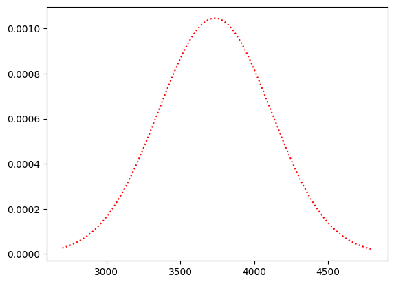
We can use a Scipy statistics distribution to make a normal distribution with the same mean and standard deviation.

import scipy.stats as sps

# A normal distribution with the same mean and standard deviation.
chinstrap_dist = sps.norm(bm_params.loc['Chinstrap', 'mean'],
                          bm_params.loc['Chinstrap', 'std'])

# The probability density function of the distribution:
chinstraps = bm_by_species.get_group('Chinstrap')
c_masses_x = np.linspace(chinstraps.min(), chinstraps.max(), 1000)
plt.plot(c_masses_x, chinstrap_dist.pdf(c_masses_x), 'r:')

[<matplotlib.lines.Line2D at 0x7f5ed9acd7d0>]

This is the plot along with the actual densities:

plt.hist(chinstraps, density=True)
plt.plot(c_masses_x, chinstrap_dist.pdf(c_masses_x), 'r:')

[<matplotlib.lines.Line2D at 0x7f5ed8647fd0>]

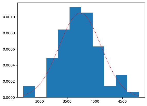
The normal (Gaussian) probability density function gives our estimate of the probability (density) of any given weight.

chinstrap_dist.pdf(3500)

np.float64(0.0008676740928442561)

With these we can get the probability of any mass in the dataset given that the penguin is a Chinstrap:

\[ P(\text{mass} | \text{Chinstrap}) \]

Actually, to be concise, let’s use \(m\) for \(\text{mass}\) and \(C\) for \(\text{Chinstrap}\).

\[ P(m | C) \]

We fill in the values of \(P(m | C)\):

df['p_m_given_c'] = chinstrap_dist.pdf(df['body_mass_g'])
df

	species	body_mass_g	bill_depth_mm	p_m_given_c
152	Gentoo	4500.0	13.2	1.386413e-04
153	Gentoo	5700.0	16.3	1.767096e-09
154	Gentoo	4450.0	14.1	1.788899e-04
155	Gentoo	5700.0	15.2	1.767096e-09
156	Gentoo	5400.0	14.5	7.477526e-08
...	...	...	...	...
339	Chinstrap	4000.0	19.8	8.186991e-04
340	Chinstrap	3400.0	18.1	7.143042e-04
341	Chinstrap	3775.0	18.2	1.039432e-03
342	Chinstrap	4100.0	19.0	6.585033e-04
343	Chinstrap	3775.0	18.7	1.039432e-03

187 rows × 4 columns

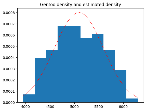
Likewise:

\[ P(\text{mass}|\text{Gentoo}) \]

which we will write as:

\[ P(m | G) \]

gentoo_dist = sps.norm(bm_params.loc['Gentoo', 'mean'],
                       bm_params.loc['Gentoo', 'std'])
gentoos = bm_by_species.get_group('Gentoo')
g_masses_x = np.linspace(gentoos.min(), gentoos.max(), 1000)
plt.hist(gentoos, density=True)
plt.plot(g_masses_x, gentoo_dist.pdf(g_masses_x), 'r:');
plt.title('Gentoo density and estimated density');

df['p_m_given_g'] = gentoo_dist.pdf(df['body_mass_g'])
df

	species	body_mass_g	bill_depth_mm	p_m_given_c	p_m_given_g
152	Gentoo	4500.0	13.2	1.386413e-04	0.000395
153	Gentoo	5700.0	16.3	1.767096e-09	0.000381
154	Gentoo	4450.0	14.1	1.788899e-04	0.000349
155	Gentoo	5700.0	15.2	1.767096e-09	0.000381
156	Gentoo	5400.0	14.5	7.477526e-08	0.000661
...	...	...	...	...	...
339	Chinstrap	4000.0	19.8	8.186991e-04	0.000073
340	Chinstrap	3400.0	18.1	7.143042e-04	0.000003
341	Chinstrap	3775.0	18.2	1.039432e-03	0.000025
342	Chinstrap	4100.0	19.0	6.585033e-04	0.000111
343	Chinstrap	3775.0	18.7	1.039432e-03	0.000025

187 rows × 5 columns

We also need prior probabilities for Chinstrap (\(C\)) and Gentoo (\(G\)):

\[ P(C) \]

\[ P(G) \]

Let’s just use the proportions in the dataset:

p_chinstrap = np.mean(df['species'] == 'Chinstrap')
p_chinstrap

np.float64(0.36363636363636365)

p_gentoo = np.mean(df['species'] == 'Gentoo')
p_gentoo

np.float64(0.6363636363636364)

df['p_chinstrap'] = p_chinstrap
df['p_gentoo'] = p_gentoo
df

	species	body_mass_g	bill_depth_mm	p_m_given_c	p_m_given_g	p_chinstrap	p_gentoo
152	Gentoo	4500.0	13.2	1.386413e-04	0.000395	0.363636	0.636364
153	Gentoo	5700.0	16.3	1.767096e-09	0.000381	0.363636	0.636364
154	Gentoo	4450.0	14.1	1.788899e-04	0.000349	0.363636	0.636364
155	Gentoo	5700.0	15.2	1.767096e-09	0.000381	0.363636	0.636364
156	Gentoo	5400.0	14.5	7.477526e-08	0.000661	0.363636	0.636364
...	...	...	...	...	...	...	...
339	Chinstrap	4000.0	19.8	8.186991e-04	0.000073	0.363636	0.636364
340	Chinstrap	3400.0	18.1	7.143042e-04	0.000003	0.363636	0.636364
341	Chinstrap	3775.0	18.2	1.039432e-03	0.000025	0.363636	0.636364
342	Chinstrap	4100.0	19.0	6.585033e-04	0.000111	0.363636	0.636364
343	Chinstrap	3775.0	18.7	1.039432e-03	0.000025	0.363636	0.636364

187 rows × 7 columns

In our model, each individual mass can only come about in one of two situations: the penguin is a Chinstrap, or the penguin is a Gentoo. That is, the mass can only come about in these situations:

\[ P(m \text{ and } C) \]

or:

\[ P(m \text{ and } G) \]

But:

\[ P(m \text{ and } C) = P(m | C) P(C) \]

and

\[ P(m \text{ and } G) = P(m | G) P(G) \]

Let’s calculate those now:

df['p_m_and_c'] = df['p_m_given_c'] * df['p_chinstrap']
df['p_m_and_g'] = df['p_m_given_g'] * df['p_gentoo']

\(P(m \text{ and } C)\), \(P(m \text{ and } G)\) are mutually exclusive, so we add the probabilities to give the probability of getting a particular mass value \(m\):

\[ P(m) = P(m \text{ and } C) + P(m \text{ and } G) \]

df['p_mass'] = df['p_m_and_c'] + df['p_m_and_g']
df

	species	body_mass_g	bill_depth_mm	p_m_given_c	p_m_given_g	p_chinstrap	p_gentoo	p_m_and_c	p_m_and_g	p_mass
152	Gentoo	4500.0	13.2	1.386413e-04	0.000395	0.363636	0.636364	5.041503e-05	0.000252	0.000302
153	Gentoo	5700.0	16.3	1.767096e-09	0.000381	0.363636	0.636364	6.425805e-10	0.000243	0.000243
154	Gentoo	4450.0	14.1	1.788899e-04	0.000349	0.363636	0.636364	6.505088e-05	0.000222	0.000287
155	Gentoo	5700.0	15.2	1.767096e-09	0.000381	0.363636	0.636364	6.425805e-10	0.000243	0.000243
156	Gentoo	5400.0	14.5	7.477526e-08	0.000661	0.363636	0.636364	2.719100e-08	0.000421	0.000421
...	...	...	...	...	...	...	...	...	...	...
339	Chinstrap	4000.0	19.8	8.186991e-04	0.000073	0.363636	0.636364	2.977088e-04	0.000046	0.000344
340	Chinstrap	3400.0	18.1	7.143042e-04	0.000003	0.363636	0.636364	2.597470e-04	0.000002	0.000261
341	Chinstrap	3775.0	18.2	1.039432e-03	0.000025	0.363636	0.636364	3.779754e-04	0.000016	0.000394
342	Chinstrap	4100.0	19.0	6.585033e-04	0.000111	0.363636	0.636364	2.394557e-04	0.000071	0.000310
343	Chinstrap	3775.0	18.7	1.039432e-03	0.000025	0.363636	0.636364	3.779754e-04	0.000016	0.000394

187 rows × 10 columns

How we have everything we need to work out the posterior probability that a penguin is a Chinstrap, given the weight of the penguin:

\[ P(C | m) = \frac{P(m | C) * P(C)}{P(m)} \]

df['p_c_given_m'] = (df['p_m_given_c'] * df['p_chinstrap']) / df['p_mass']
df

	species	body_mass_g	bill_depth_mm	p_m_given_c	p_m_given_g	p_chinstrap	p_gentoo	p_m_and_c	p_m_and_g	p_mass	p_c_given_m
152	Gentoo	4500.0	13.2	1.386413e-04	0.000395	0.363636	0.636364	5.041503e-05	0.000252	0.000302	0.166976
153	Gentoo	5700.0	16.3	1.767096e-09	0.000381	0.363636	0.636364	6.425805e-10	0.000243	0.000243	0.000003
154	Gentoo	4450.0	14.1	1.788899e-04	0.000349	0.363636	0.636364	6.505088e-05	0.000222	0.000287	0.226439
155	Gentoo	5700.0	15.2	1.767096e-09	0.000381	0.363636	0.636364	6.425805e-10	0.000243	0.000243	0.000003
156	Gentoo	5400.0	14.5	7.477526e-08	0.000661	0.363636	0.636364	2.719100e-08	0.000421	0.000421	0.000065
...	...	...	...	...	...	...	...	...	...	...	...
339	Chinstrap	4000.0	19.8	8.186991e-04	0.000073	0.363636	0.636364	2.977088e-04	0.000046	0.000344	0.865038
340	Chinstrap	3400.0	18.1	7.143042e-04	0.000003	0.363636	0.636364	2.597470e-04	0.000002	0.000261	0.993768
341	Chinstrap	3775.0	18.2	1.039432e-03	0.000025	0.363636	0.636364	3.779754e-04	0.000016	0.000394	0.960216
342	Chinstrap	4100.0	19.0	6.585033e-04	0.000111	0.363636	0.636364	2.394557e-04	0.000071	0.000310	0.772415
343	Chinstrap	3775.0	18.7	1.039432e-03	0.000025	0.363636	0.636364	3.779754e-04	0.000016	0.000394	0.960216

187 rows × 11 columns

Likewise:

\[ P(G | m) = \frac{P(m | G) * P(G)}{P(m)} \]

df['p_g_given_m'] = (df['p_m_given_g'] * df['p_gentoo']) / df['p_mass']
df

	species	body_mass_g	bill_depth_mm	p_m_given_c	p_m_given_g	p_chinstrap	p_gentoo	p_m_and_c	p_m_and_g	p_mass	p_c_given_m	p_g_given_m
152	Gentoo	4500.0	13.2	1.386413e-04	0.000395	0.363636	0.636364	5.041503e-05	0.000252	0.000302	0.166976	0.833024
153	Gentoo	5700.0	16.3	1.767096e-09	0.000381	0.363636	0.636364	6.425805e-10	0.000243	0.000243	0.000003	0.999997
154	Gentoo	4450.0	14.1	1.788899e-04	0.000349	0.363636	0.636364	6.505088e-05	0.000222	0.000287	0.226439	0.773561
155	Gentoo	5700.0	15.2	1.767096e-09	0.000381	0.363636	0.636364	6.425805e-10	0.000243	0.000243	0.000003	0.999997
156	Gentoo	5400.0	14.5	7.477526e-08	0.000661	0.363636	0.636364	2.719100e-08	0.000421	0.000421	0.000065	0.999935
...	...	...	...	...	...	...	...	...	...	...	...	...
339	Chinstrap	4000.0	19.8	8.186991e-04	0.000073	0.363636	0.636364	2.977088e-04	0.000046	0.000344	0.865038	0.134962
340	Chinstrap	3400.0	18.1	7.143042e-04	0.000003	0.363636	0.636364	2.597470e-04	0.000002	0.000261	0.993768	0.006232
341	Chinstrap	3775.0	18.2	1.039432e-03	0.000025	0.363636	0.636364	3.779754e-04	0.000016	0.000394	0.960216	0.039784
342	Chinstrap	4100.0	19.0	6.585033e-04	0.000111	0.363636	0.636364	2.394557e-04	0.000071	0.000310	0.772415	0.227585
343	Chinstrap	3775.0	18.7	1.039432e-03	0.000025	0.363636	0.636364	3.779754e-04	0.000016	0.000394	0.960216	0.039784

187 rows × 12 columns

df['bayes_predictions'] = np.where(
    df['p_c_given_m'] > df['p_g_given_m'],
    'Chinstrap', 'Gentoo')
df

	species	body_mass_g	bill_depth_mm	p_m_given_c	p_m_given_g	p_chinstrap	p_gentoo	p_m_and_c	p_m_and_g	p_mass	p_c_given_m	p_g_given_m	bayes_predictions
152	Gentoo	4500.0	13.2	1.386413e-04	0.000395	0.363636	0.636364	5.041503e-05	0.000252	0.000302	0.166976	0.833024	Gentoo
153	Gentoo	5700.0	16.3	1.767096e-09	0.000381	0.363636	0.636364	6.425805e-10	0.000243	0.000243	0.000003	0.999997	Gentoo
154	Gentoo	4450.0	14.1	1.788899e-04	0.000349	0.363636	0.636364	6.505088e-05	0.000222	0.000287	0.226439	0.773561	Gentoo
155	Gentoo	5700.0	15.2	1.767096e-09	0.000381	0.363636	0.636364	6.425805e-10	0.000243	0.000243	0.000003	0.999997	Gentoo
156	Gentoo	5400.0	14.5	7.477526e-08	0.000661	0.363636	0.636364	2.719100e-08	0.000421	0.000421	0.000065	0.999935	Gentoo
...	...	...	...	...	...	...	...	...	...	...	...	...	...
339	Chinstrap	4000.0	19.8	8.186991e-04	0.000073	0.363636	0.636364	2.977088e-04	0.000046	0.000344	0.865038	0.134962	Chinstrap
340	Chinstrap	3400.0	18.1	7.143042e-04	0.000003	0.363636	0.636364	2.597470e-04	0.000002	0.000261	0.993768	0.006232	Chinstrap
341	Chinstrap	3775.0	18.2	1.039432e-03	0.000025	0.363636	0.636364	3.779754e-04	0.000016	0.000394	0.960216	0.039784	Chinstrap
342	Chinstrap	4100.0	19.0	6.585033e-04	0.000111	0.363636	0.636364	2.394557e-04	0.000071	0.000310	0.772415	0.227585	Chinstrap
343	Chinstrap	3775.0	18.7	1.039432e-03	0.000025	0.363636	0.636364	3.779754e-04	0.000016	0.000394	0.960216	0.039784	Chinstrap

187 rows × 13 columns

But - wait - for our Bayes predictions, we don’t actually need the \(P(\text{mass})\) value. Why? Because we can calculate the ratio of the posterior probabilities like this:

\[\begin{split} \text{LR} = \frac{P(C | m)}{P(G | m)} \\ = \frac {\frac{ P(m | C) * P(C) } { P(m) }} {\frac{P(m | G) * P(G)} { P(m) }} \\ = \frac{P(m | C) * P(C)} {P(m | G) * P(G)} \end{split}\]

likelihood_ratio = ((df['p_m_given_c'] * df['p_chinstrap']) /
                    (df['p_m_given_g'] * df['p_gentoo']))

# From the divide-out trick above, this gives us the same as:
np.allclose(likelihood_ratio, df['p_c_given_m'] / df['p_g_given_m'])

True

Notice we have divided out the \(P(\text{mass})\) in this ratio. Notice too that ratios above 1 mean more likely Chinstrap, and less than one mean less likely Chinstrap, more likely Gentoo. So we get the same predictions from the likelihood as we would from the full posterior probabilities:

likelihood_predictions = np.where(
    likelihood_ratio > 1,
    'Chinstrap', 'Gentoo')
np.all(df['bayes_predictions'] == likelihood_predictions)

np.True_

As you may remember from the logit transform in logistic regression, we can also get probabilities from the likelihood ratios, with:

# Probability from likelihood ratio
p_from_lr = likelihood_ratio / (1 + likelihood_ratio)
p_from_lr

152    0.166976
153    0.000003
154    0.226439
155    0.000003
156    0.000065
         ...   
339    0.865038
340    0.993768
341    0.960216
342    0.772415
343    0.960216
Length: 187, dtype: float64

Here is the same process, using the Scikit-learn library.

from sklearn.naive_bayes import GaussianNB
model = GaussianNB()
model.fit(df[['body_mass_g']], df['species']);
model.class_prior_

array([0.36363636, 0.63636364])

df['sklearn_predictions'] = model.predict(df[['body_mass_g']])
df

	species	body_mass_g	bill_depth_mm	p_m_given_c	p_m_given_g	p_chinstrap	p_gentoo	p_m_and_c	p_m_and_g	p_mass	p_c_given_m	p_g_given_m	bayes_predictions	sklearn_predictions
152	Gentoo	4500.0	13.2	1.386413e-04	0.000395	0.363636	0.636364	5.041503e-05	0.000252	0.000302	0.166976	0.833024	Gentoo	Gentoo
153	Gentoo	5700.0	16.3	1.767096e-09	0.000381	0.363636	0.636364	6.425805e-10	0.000243	0.000243	0.000003	0.999997	Gentoo	Gentoo
154	Gentoo	4450.0	14.1	1.788899e-04	0.000349	0.363636	0.636364	6.505088e-05	0.000222	0.000287	0.226439	0.773561	Gentoo	Gentoo
155	Gentoo	5700.0	15.2	1.767096e-09	0.000381	0.363636	0.636364	6.425805e-10	0.000243	0.000243	0.000003	0.999997	Gentoo	Gentoo
156	Gentoo	5400.0	14.5	7.477526e-08	0.000661	0.363636	0.636364	2.719100e-08	0.000421	0.000421	0.000065	0.999935	Gentoo	Gentoo
...	...	...	...	...	...	...	...	...	...	...	...	...	...	...
339	Chinstrap	4000.0	19.8	8.186991e-04	0.000073	0.363636	0.636364	2.977088e-04	0.000046	0.000344	0.865038	0.134962	Chinstrap	Chinstrap
340	Chinstrap	3400.0	18.1	7.143042e-04	0.000003	0.363636	0.636364	2.597470e-04	0.000002	0.000261	0.993768	0.006232	Chinstrap	Chinstrap
341	Chinstrap	3775.0	18.2	1.039432e-03	0.000025	0.363636	0.636364	3.779754e-04	0.000016	0.000394	0.960216	0.039784	Chinstrap	Chinstrap
342	Chinstrap	4100.0	19.0	6.585033e-04	0.000111	0.363636	0.636364	2.394557e-04	0.000071	0.000310	0.772415	0.227585	Chinstrap	Chinstrap
343	Chinstrap	3775.0	18.7	1.039432e-03	0.000025	0.363636	0.636364	3.779754e-04	0.000016	0.000394	0.960216	0.039784	Chinstrap	Chinstrap

187 rows × 14 columns

Scikit-learn gives the same predictions as we do:

np.all(df['bayes_predictions'] == df['sklearn_predictions'])

np.True_

Scikit-learn also calculates the posterior probabilities:

# The predict_proba values are just the posteriors.
skl_posteriors = model.predict_proba(df[['body_mass_g']])
# They are the same as ours, with calculation error.
our_posteriors = df[['p_c_given_m', 'p_g_given_m']]
assert np.allclose(skl_posteriors, our_posteriors)

The score is the proportion of labels we predicted correctly:

model.score(df[['body_mass_g']], df['species'])

0.9358288770053476

Here we calculated the same value by hand(ish):

np.mean(df['sklearn_predictions'] == df['species'])

np.float64(0.9358288770053476)

Putting the naïve into “naïve Bayes”

Now, let’s also consider the bill_depth_mm values:

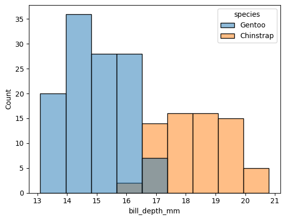
sns.histplot(data=df, x="bill_depth_mm", hue="species")

<Axes: xlabel='bill_depth_mm', ylabel='Count'>

Make the distributions for bill depth:

bd_by_species = by_species['bill_depth_mm']
bd_params = bd_by_species.agg(mean='mean', std=lambda x : np.std(x))
# The distributions
pd_dists = {}
species = ['Chinstrap', 'Gentoo']
for name in species:
    pd_dists[name] = sps.norm(bd_params.loc[name, 'mean'],
                              bd_params.loc[name, 'std'])

pd_dists

{'Chinstrap': <scipy.stats._distn_infrastructure.rv_continuous_frozen at 0x7f5ed1a22990>,
 'Gentoo': <scipy.stats._distn_infrastructure.rv_continuous_frozen at 0x7f5ed8674f90>}

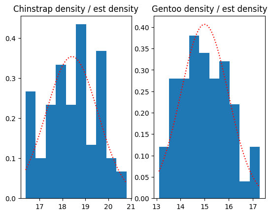
Plot the actual and estimated density, using the Gaussian approximations:

fig, axes = plt.subplots(1, 2)
for i, name in enumerate(species):
    axis = axes[i]
    bds = bd_by_species.get_group(name)
    x = np.linspace(bds.min(), bds.max(), 1000)
    axis.hist(bds, density=True)
    axis.plot(x, pd_dists[name].pdf(x), 'r:');
    axis.set_title(f'{name} density / est density')

We can also think of these distributions in two dimensions, along with the mass:

sns.scatterplot(df, x='body_mass_g', y='bill_depth_mm',
                hue='species')

<Axes: xlabel='body_mass_g', ylabel='bill_depth_mm'>

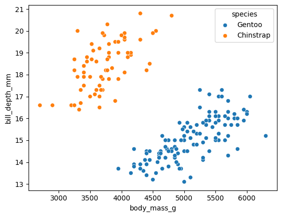
Question - is the bill depth independent (in the sense of probability) from the body mass? That is - if I know the body mass, do I know anything more about the bill depth?

For the moment - let’s say “yes” (it’s independent). That’s naïve. And that’s where “naïve” Bayes reaches the name of the technique.

Using independence, we can calculate the probability of a combination of a particular body mass and bill depth value.

Call \(P(d)\) the probability of a particular bill depth value. Naïve Bayes estimates the probability of the combination with:

\[ P((m \text{ and } d) | C) = P(m | C) * P(d | C) \]

Let’s calculate the new probabilities we need:

df['p_bd_given_c'] = pd_dists['Chinstrap'].pdf(df['bill_depth_mm'])
df['p_bd_given_g'] = pd_dists['Gentoo'].pdf(df['bill_depth_mm'])
df

	species	body_mass_g	bill_depth_mm	p_m_given_c	p_m_given_g	p_chinstrap	p_gentoo	p_m_and_c	p_m_and_g	p_mass	p_c_given_m	p_g_given_m	bayes_predictions	sklearn_predictions	p_bd_given_c	p_bd_given_g
152	Gentoo	4500.0	13.2	1.386413e-04	0.000395	0.363636	0.636364	5.041503e-05	0.000252	0.000302	0.166976	0.833024	Gentoo	Gentoo	0.000008	0.076169
153	Gentoo	5700.0	16.3	1.767096e-09	0.000381	0.363636	0.636364	6.425805e-10	0.000243	0.000243	0.000003	0.999997	Gentoo	Gentoo	0.060282	0.168353
154	Gentoo	4450.0	14.1	1.788899e-04	0.000349	0.363636	0.636364	6.505088e-05	0.000222	0.000287	0.226439	0.773561	Gentoo	Gentoo	0.000228	0.267777
155	Gentoo	5700.0	15.2	1.767096e-09	0.000381	0.363636	0.636364	6.425805e-10	0.000243	0.000243	0.000003	0.999997	Gentoo	Gentoo	0.005967	0.397696
156	Gentoo	5400.0	14.5	7.477526e-08	0.000661	0.363636	0.636364	2.719100e-08	0.000421	0.000421	0.000065	0.999935	Gentoo	Gentoo	0.000834	0.357527
...	...	...	...	...	...	...	...	...	...	...	...	...	...	...	...	...
339	Chinstrap	4000.0	19.8	8.186991e-04	0.000073	0.363636	0.636364	2.977088e-04	0.000046	0.000344	0.865038	0.134962	Chinstrap	Chinstrap	0.167371	0.000003
340	Chinstrap	3400.0	18.1	7.143042e-04	0.000003	0.363636	0.636364	2.597470e-04	0.000002	0.000261	0.993768	0.006232	Chinstrap	Chinstrap	0.339946	0.002751
341	Chinstrap	3775.0	18.2	1.039432e-03	0.000025	0.363636	0.636364	3.779754e-04	0.000016	0.000394	0.960216	0.039784	Chinstrap	Chinstrap	0.347265	0.001984
342	Chinstrap	4100.0	19.0	6.585033e-04	0.000111	0.363636	0.636364	2.394557e-04	0.000071	0.000310	0.772415	0.227585	Chinstrap	Chinstrap	0.310160	0.000100
343	Chinstrap	3775.0	18.7	1.039432e-03	0.000025	0.363636	0.636364	3.779754e-04	0.000016	0.000394	0.960216	0.039784	Chinstrap	Chinstrap	0.343268	0.000331

187 rows × 16 columns

The full formula for the posterior using the two measures is:

\[ P(C | (m \text{ and } d)) = \frac{ P((m \text{ and } d) | C) * P(C) }{P(m \text{ and } d)} \]

The naïve version of the formula is:

\[ P(C | (m \text{ and } d)) = \frac{ P(m | C) * P(d | C) * P(C) }{P(m \text{ and } d)} \]

But - using the likelihood trick above, we no longer have to calculate the denominator, we can just divide it out, to give the following ratio:

both_ratio = ((df['p_m_given_c'] * df['p_bd_given_c'] * df['p_chinstrap']) /
              (df['p_m_given_g'] * df['p_bd_given_g'] * df['p_gentoo']))
df['both_predictions'] = np.where(both_ratio > 1, 'Chinstrap', 'Gentoo')
df

	species	body_mass_g	bill_depth_mm	p_m_given_c	p_m_given_g	p_chinstrap	p_gentoo	p_m_and_c	p_m_and_g	p_mass	p_c_given_m	p_g_given_m	bayes_predictions	sklearn_predictions	p_bd_given_c	p_bd_given_g	both_predictions
152	Gentoo	4500.0	13.2	1.386413e-04	0.000395	0.363636	0.636364	5.041503e-05	0.000252	0.000302	0.166976	0.833024	Gentoo	Gentoo	0.000008	0.076169	Gentoo
153	Gentoo	5700.0	16.3	1.767096e-09	0.000381	0.363636	0.636364	6.425805e-10	0.000243	0.000243	0.000003	0.999997	Gentoo	Gentoo	0.060282	0.168353	Gentoo
154	Gentoo	4450.0	14.1	1.788899e-04	0.000349	0.363636	0.636364	6.505088e-05	0.000222	0.000287	0.226439	0.773561	Gentoo	Gentoo	0.000228	0.267777	Gentoo
155	Gentoo	5700.0	15.2	1.767096e-09	0.000381	0.363636	0.636364	6.425805e-10	0.000243	0.000243	0.000003	0.999997	Gentoo	Gentoo	0.005967	0.397696	Gentoo
156	Gentoo	5400.0	14.5	7.477526e-08	0.000661	0.363636	0.636364	2.719100e-08	0.000421	0.000421	0.000065	0.999935	Gentoo	Gentoo	0.000834	0.357527	Gentoo
...	...	...	...	...	...	...	...	...	...	...	...	...	...	...	...	...	...
339	Chinstrap	4000.0	19.8	8.186991e-04	0.000073	0.363636	0.636364	2.977088e-04	0.000046	0.000344	0.865038	0.134962	Chinstrap	Chinstrap	0.167371	0.000003	Chinstrap
340	Chinstrap	3400.0	18.1	7.143042e-04	0.000003	0.363636	0.636364	2.597470e-04	0.000002	0.000261	0.993768	0.006232	Chinstrap	Chinstrap	0.339946	0.002751	Chinstrap
341	Chinstrap	3775.0	18.2	1.039432e-03	0.000025	0.363636	0.636364	3.779754e-04	0.000016	0.000394	0.960216	0.039784	Chinstrap	Chinstrap	0.347265	0.001984	Chinstrap
342	Chinstrap	4100.0	19.0	6.585033e-04	0.000111	0.363636	0.636364	2.394557e-04	0.000071	0.000310	0.772415	0.227585	Chinstrap	Chinstrap	0.310160	0.000100	Chinstrap
343	Chinstrap	3775.0	18.7	1.039432e-03	0.000025	0.363636	0.636364	3.779754e-04	0.000016	0.000394	0.960216	0.039784	Chinstrap	Chinstrap	0.343268	0.000331	Chinstrap

187 rows × 17 columns

Accuracy:

np.mean(df['both_predictions'] == df['species'])

np.float64(1.0)

Scikit learn:

both_model = GaussianNB()
both_model.fit(df[['body_mass_g', 'bill_depth_mm']], df['species'])

GaussianNB()

In a Jupyter environment, please rerun this cell to show the HTML representation or trust the notebook.
On GitHub, the HTML representation is unable to render, please try loading this page with nbviewer.org.

both_model.score(df[['body_mass_g', 'bill_depth_mm']], df['species'])

1.0

Let’s try the standard test-train split. We “train” our classifier using a random subset of the data:

from sklearn.model_selection import train_test_split

X_train, X_test, y_train, y_test = train_test_split(
    df[['body_mass_g', 'bill_depth_mm']],
    df['species'])
X_train

	body_mass_g	bill_depth_mm
210	4450.0	14.5
310	3600.0	18.6
241	5550.0	17.0
208	4300.0	13.9
295	4400.0	18.2
...	...	...
282	3250.0	18.2
249	4875.0	14.6
219	5800.0	16.2
184	5050.0	14.5
167	5850.0	15.7

140 rows × 2 columns

Here we fit the various parameters to classify the training data.

test_model = GaussianNB()
test_model.fit(X_train, y_train)

GaussianNB()

In a Jupyter environment, please rerun this cell to show the HTML representation or trust the notebook.
On GitHub, the HTML representation is unable to render, please try loading this page with nbviewer.org.

How does Scikit-learn do in classifying the test data (that it has not seen before):

test_model.score(X_test, y_test)

1.0

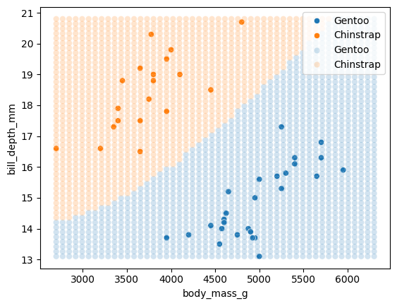
We can look at the decision boundary to see where the model starts seeing Chinstrap and Gentoo penguins, as it moves through the 2D space of parameters (mass and bill depth).

# Make grid of points to classify
all_params = df[['body_mass_g', 'bill_depth_mm']].describe()
bm_x = np.linspace(all_params.loc['min', 'body_mass_g'],
                   all_params.loc['max', 'body_mass_g'],
                   50)
bm_y = np.linspace(all_params.loc['min', 'bill_depth_mm'],
                   all_params.loc['max', 'bill_depth_mm'],
                   50)
x, y = np.meshgrid(bm_x, bm_y)
xy = np.stack((x.ravel(), y.ravel()), axis=1)
xy_df = pd.DataFrame(xy, columns=X_test.columns)

# Show the classification of the test data.
sns.scatterplot(df.loc[X_test.index],
                x='body_mass_g', y='bill_depth_mm',
                hue='species')
# Overlay the classification of the grid points.
sns.scatterplot(x=xy[:, 0], y=xy[:, 1],
                hue=test_model.predict(xy_df),
                palette=sns.color_palette()[:2],
                alpha=0.2);