k-means clustering#
Also see: k-means clustering in the Python Data Science Handbook. You’ll see much inspiration from that page here.
import numpy as np
import pandas as pd
pd.set_option('mode.copy_on_write', True)
import matplotlib.pyplot as plt
import seaborn as sns
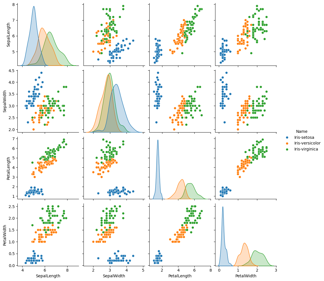
We will use the famous iris data set. Quoting from the Wikipedia page above:
The data set consists of 50 samples from each of three species of Iris (Iris setosa, Iris virginica and Iris versicolor). Four features were measured from each sample: the length and the width of the sepals and petals, in centimeters.
iris = pd.read_csv('data/iris.csv')
iris
| SepalLength | SepalWidth | PetalLength | PetalWidth | Name | |
|---|---|---|---|---|---|
| 0 | 5.1 | 3.5 | 1.4 | 0.2 | Iris-setosa |
| 1 | 4.9 | 3.0 | 1.4 | 0.2 | Iris-setosa |
| 2 | 4.7 | 3.2 | 1.3 | 0.2 | Iris-setosa |
| 3 | 4.6 | 3.1 | 1.5 | 0.2 | Iris-setosa |
| 4 | 5.0 | 3.6 | 1.4 | 0.2 | Iris-setosa |
| ... | ... | ... | ... | ... | ... |
| 145 | 6.7 | 3.0 | 5.2 | 2.3 | Iris-virginica |
| 146 | 6.3 | 2.5 | 5.0 | 1.9 | Iris-virginica |
| 147 | 6.5 | 3.0 | 5.2 | 2.0 | Iris-virginica |
| 148 | 6.2 | 3.4 | 5.4 | 2.3 | Iris-virginica |
| 149 | 5.9 | 3.0 | 5.1 | 1.8 | Iris-virginica |
150 rows × 5 columns
sns.pairplot(iris, hue='Name')
<seaborn.axisgrid.PairGrid at 0x7fe2763c3b50>
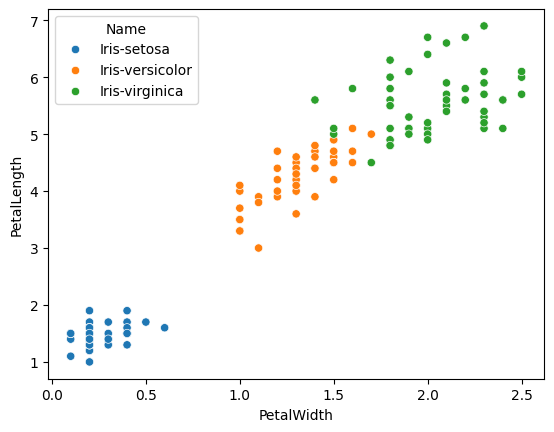
features = ['PetalWidth', 'PetalLength']
measures = iris[features]
measures
| PetalWidth | PetalLength | |
|---|---|---|
| 0 | 0.2 | 1.4 |
| 1 | 0.2 | 1.4 |
| 2 | 0.2 | 1.3 |
| 3 | 0.2 | 1.5 |
| 4 | 0.2 | 1.4 |
| ... | ... | ... |
| 145 | 2.3 | 5.2 |
| 146 | 1.9 | 5.0 |
| 147 | 2.0 | 5.2 |
| 148 | 2.3 | 5.4 |
| 149 | 1.8 | 5.1 |
150 rows × 2 columns
sns.scatterplot(iris,
                x=features[0],
                y=features[1],
                hue='Name')
<Axes: xlabel='PetalWidth', ylabel='PetalLength'>
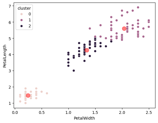
K-means is a technique for splitting up (classifying) the data into clusters — groups of nearby points. Here is Scikit-learn’s k-means implementation. We use it to identify clusters in the data automatically, without using the species labels. We define the clusters by their centers. Notice though that the clusters it finds are very similar to the clusters by species.
from sklearn.cluster import KMeans

# n_init is the number of different starting states to try.
# The algorithm depends to some extent on starting state.
kmeans_model = KMeans(n_clusters=3, n_init=10)
kmeans_model.fit(measures)
cluster_nos = kmeans_model.predict(measures)
# The measures with Scikit-learn's cluster labels.
labeled_measures = measures.copy()
labeled_measures['cluster'] = cluster_nos
labeled_measures
| PetalWidth | PetalLength | cluster | |
|---|---|---|---|
| 0 | 0.2 | 1.4 | 0 |
| 1 | 0.2 | 1.4 | 0 |
| 2 | 0.2 | 1.3 | 0 |
| 3 | 0.2 | 1.5 | 0 |
| 4 | 0.2 | 1.4 | 0 |
| ... | ... | ... | ... |
| 145 | 2.3 | 5.2 | 1 |
| 146 | 1.9 | 5.0 | 1 |
| 147 | 2.0 | 5.2 | 1 |
| 148 | 2.3 | 5.4 | 1 |
| 149 | 1.8 | 5.1 | 1 |
150 rows × 3 columns
These are Scikit-learn’s cluster centers:
kmeans_model.cluster_centers_
array([[0.244     , 1.464     ],
       [2.0375    , 5.59583333],
       [1.34230769, 4.26923077]])
The clusters displayed graphically. Notice how similar they are to the actual species labels, that we have not used here.
sns.scatterplot(labeled_measures,
                x=features[0],
                y=features[1],
                hue='cluster')
plt.scatter(kmeans_model.cluster_centers_[:, 0],
            kmeans_model.cluster_centers_[:, 1],
            color='r', s=100, alpha=0.5);
The algorithm of k-means is as follows. We specify we want \(k\) clusters, then:
Select \(k\) points at random from the set to be the starting estimates of the cluster centers.
Repeat the following until the cluster center estimates do not change:
A. Calculate the distance of each point in the dataset to each of the \(k\) clusters.
B. Allocate each point to one of the clusters by choosing the cluster with the shortest distance to the point.
C. With these allocations, calculate new estimated cluster centers by averaging the positions of all points in each cluster.
D. Check if the new cluster centers estimate has changed. If not we are finished.
Remember the loop here as:
A. Calculate the distance.
B. Allocate each point to one the centers.
C. Calculate new centers.
D. Check.
# Step 1: Select k points at random as starting estimates.
n_clusters = 3
cluster_names = np.array(['c0', 'c1', 'c2'])
df = iris[features]
# .sample does sampling without replacement by default.
centers = df.sample(n_clusters).set_index(cluster_names)
centers
| PetalWidth | PetalLength | |
|---|---|---|
| c0 | 1.0 | 3.7 |
| c1 | 0.2 | 1.9 |
| c2 | 1.9 | 5.1 |
This is step 2A - calculate the distance of each point to each each center.
def distance(pt1, pt2):
    return np.sqrt(np.sum((pt1 - pt2) ** 2))
# An example distance.
distance(df.iloc[0], centers.iloc[0])
np.float64(2.4351591323771844)
Calculate the distances between all clusters and all points:
distances = pd.DataFrame()
# Distances of all points to cluster center 0
distances['c0'] = df.apply(
    distance,
    pt2=centers.iloc[0],
    axis=1)
# Distances of all points to cluster center 1
distances['c1'] = df.apply(
    distance,
    pt2=centers.iloc[1],
    axis=1)
# Distances of all points to cluster center 2
distances['c2'] = df.apply(
    distance,
    pt2=centers.iloc[2],
    axis=1)
distances
| c0 | c1 | c2 | |
|---|---|---|---|
| 0 | 2.435159 | 0.500000 | 4.071855 |
| 1 | 2.435159 | 0.500000 | 4.071855 |
| 2 | 2.529822 | 0.600000 | 4.162932 |
| 3 | 2.340940 | 0.400000 | 3.981206 |
| 4 | 2.435159 | 0.500000 | 4.071855 |
| ... | ... | ... | ... |
| 145 | 1.984943 | 3.911521 | 0.412311 |
| 146 | 1.581139 | 3.535534 | 0.100000 |
| 147 | 1.802776 | 3.758989 | 0.141421 |
| 148 | 2.140093 | 4.081666 | 0.500000 |
| 149 | 1.612452 | 3.577709 | 0.100000 |
150 rows × 3 columns
# We can write the code above in a more compact way.
distances = pd.DataFrame()
for point_no, cluster_name in enumerate(cluster_names):
    distances[cluster_name] = df.apply(
        distance,
        pt2=centers.iloc[point_no],
        axis=1)
distances
| c0 | c1 | c2 | |
|---|---|---|---|
| 0 | 2.435159 | 0.500000 | 4.071855 |
| 1 | 2.435159 | 0.500000 | 4.071855 |
| 2 | 2.529822 | 0.600000 | 4.162932 |
| 3 | 2.340940 | 0.400000 | 3.981206 |
| 4 | 2.435159 | 0.500000 | 4.071855 |
| ... | ... | ... | ... |
| 145 | 1.984943 | 3.911521 | 0.412311 |
| 146 | 1.581139 | 3.535534 | 0.100000 |
| 147 | 1.802776 | 3.758989 | 0.141421 |
| 148 | 2.140093 | 4.081666 | 0.500000 |
| 149 | 1.612452 | 3.577709 | 0.100000 |
150 rows × 3 columns
Here are the points and the distances of the points from the three current center estimates:
pd.concat([df, distances], axis=1).round(4)
| PetalWidth | PetalLength | c0 | c1 | c2 | |
|---|---|---|---|---|---|
| 0 | 0.2 | 1.4 | 2.4352 | 0.5000 | 4.0719 |
| 1 | 0.2 | 1.4 | 2.4352 | 0.5000 | 4.0719 |
| 2 | 0.2 | 1.3 | 2.5298 | 0.6000 | 4.1629 |
| 3 | 0.2 | 1.5 | 2.3409 | 0.4000 | 3.9812 |
| 4 | 0.2 | 1.4 | 2.4352 | 0.5000 | 4.0719 |
| ... | ... | ... | ... | ... | ... |
| 145 | 2.3 | 5.2 | 1.9849 | 3.9115 | 0.4123 |
| 146 | 1.9 | 5.0 | 1.5811 | 3.5355 | 0.1000 |
| 147 | 2.0 | 5.2 | 1.8028 | 3.7590 | 0.1414 |
| 148 | 2.3 | 5.4 | 2.1401 | 4.0817 | 0.5000 |
| 149 | 1.8 | 5.1 | 1.6125 | 3.5777 | 0.1000 |
150 rows × 5 columns
Step 2B - allocate each point to a cluster. Now we can choose a cluster for each point, by choosing the cluster center with the shortest distance to the point.
# Step 2B - allocate each point to a cluster by choosing nearest center
labels = distances.idxmin(axis=1)
labels
0      c1
1      c1
2      c1
3      c1
4      c1
       ..
145    c2
146    c2
147    c2
148    c2
149    c2
Length: 150, dtype: object
Step 2C - calculate new estimated cluster centers. We estimate new cluster centers by taking the average of the point coordinates, for the points we have just allocated to each cluster.
new_centers = df.groupby(labels).mean().set_index(cluster_names)
new_centers
| PetalWidth | PetalLength | |
|---|---|---|
| c0 | 1.210345 | 3.955172 |
| c1 | 0.244000 | 1.464000 |
| c2 | 1.866197 | 5.294366 |
The next step (2D) is to check whether centers and new_centers are the
same - in which case, we have finished the search, and we can stop.
Now let’s run the whole search procedure.
# Make a new random number generator with known state.
# We do this to make sure we get the optimum k-means
# "by accident" on the first run.
rng2 = np.random.default_rng(42)
# Choose random points from set.
centers = df.sample(n_clusters,
                    random_state=rng2  # Use predictable rng
                   ).set_index(cluster_names)

# Repeat for a long time, if necessary.
for i in range(1000):

    # Find distances of each point to each center.
    distances = pd.DataFrame()
    for point_no, cluster_name in enumerate(cluster_names):
        distances[cluster_name] = df.apply(
            distance,
            pt2=centers.iloc[point_no],
            axis=1)
    # Allocate each point to one of the cluster (centers) by
    # choosing the closest center.
    labels = distances.idxmin(axis=1)

    # Make new centers with mean of points in cluster.
    new_centers = df.groupby(labels).mean().set_index(cluster_names)

    # See if we have the same centers as before.
    if np.all(centers == new_centers):
        break  # If same, then stop, we've finished.
    # Otherwise continue
    centers = new_centers
    # Show the current estimated centers.
    print(f'Centers after iteration {i}')
    display(centers)
Centers after iteration 0
| PetalWidth | PetalLength | |
|---|---|---|
| c0 | 1.192308 | 3.903846 |
| c1 | 0.244000 | 1.464000 |
| c2 | 1.845946 | 5.258108 |
Centers after iteration 1
| PetalWidth | PetalLength | |
|---|---|---|
| c0 | 1.266667 | 4.105128 |
| c1 | 0.244000 | 1.464000 |
| c2 | 1.937705 | 5.418033 |
Centers after iteration 2
| PetalWidth | PetalLength | |
|---|---|---|
| c0 | 1.302174 | 4.191304 |
| c1 | 0.244000 | 1.464000 |
| c2 | 1.994444 | 5.514815 |
Centers after iteration 3
| PetalWidth | PetalLength | |
|---|---|---|
| c0 | 1.310417 | 4.220833 |
| c1 | 0.244000 | 1.464000 |
| c2 | 2.013462 | 5.538462 |
Centers after iteration 4
| PetalWidth | PetalLength | |
|---|---|---|
| c0 | 1.339216 | 4.254902 |
| c1 | 0.244000 | 1.464000 |
| c2 | 2.026531 | 5.583673 |
Centers after iteration 5
| PetalWidth | PetalLength | |
|---|---|---|
| c0 | 1.342308 | 4.269231 |
| c1 | 0.244000 | 1.464000 |
| c2 | 2.037500 | 5.595833 |
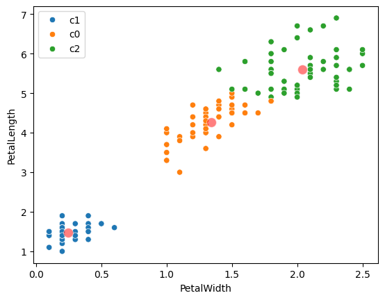
# Plot the points with their cluster labels.
sns.scatterplot(
    df,
    x=features[0],
    y=features[1],
    hue=labels)
# Plot the centers.
sns.scatterplot(
    centers,
    x=features[0],
    y=features[1],
    color='r',
    s=100,
    alpha=0.5);
centers
| PetalWidth | PetalLength | |
|---|---|---|
| c0 | 1.342308 | 4.269231 |
| c1 | 0.244000 | 1.464000 |
| c2 | 2.037500 | 5.595833 |
Notice that the centers we found are the same as those that scikit-learn found. Scikit-learn uses some tricks to make sure it found the right centers - that it didn’t get stuck with some wrong starting points. We cheated to make sure of this above, by setting the random number generator.
kmeans_model.cluster_centers_
array([[0.244     , 1.464     ],
       [2.0375    , 5.59583333],
       [1.34230769, 4.26923077]])
# Scikit-learn clusters are (near as dammit) the same as
# the ones we found.  The order of the centers is arbitrary,
# solve by sorting.
assert np.allclose(
    np.sort(kmeans_model.cluster_centers_, axis=0),
    np.sort(centers, axis=0))
One measure of how well the points match the clusters is inertia - the sum of the squared distances between each point and its corresponding cluster.
def center_difference_sq(sub_df):
    """ Squared difference between each point and matching center
    """
    return (sub_df - sub_df.mean(axis=0)) ** 2
# .transform applies the function to each sub-dataframe.
df.groupby(labels).transform(center_difference_sq).sum().sum()
np.float64(31.387758974358974)
Scikit-learn does the same calculation.
kmeans_model.inertia_
31.38775897435897